On Some Average Properties of Convex Mosaics

(1)

Full Terms & Conditions of access and use can be found at

https://www.tandfonline.com/action/journalInformation?journalCode=uexm20

Experimental Mathematics

ISSN: 1058-6458 (Print) 1944-950X (Online) Journal homepage: https://www.tandfonline.com/loi/uexm20

On Some Average Properties of Convex Mosaics

Gábor Domokos & Zsolt Lángi

To cite this article: Gábor Domokos & Zsolt Lángi (2019): On Some Average Properties of Convex Mosaics, Experimental Mathematics, DOI: 10.1080/10586458.2019.1691090

To link to this article: https://doi.org/10.1080/10586458.2019.1691090

Submit your article to this journal

Article views: 268

View related articles

View Crossmark data

(2)

On Some Average Properties of Convex Mosaics

Gabor Domokos^aand Zsolt Langi^b

aMTA-BME Morphodynamics Research Group and Dept. of Mechanics, Materials and Structures, Budapest University of Technology, Budapest, Hungary;^bMTA-BME Morphodynamics Research Group and Dept. of Geometry, Budapest University of Technology, Budapest, Hungary

ABSTRACT

In a convex mosaic inR^dwe denote the average number of vertices of a cell by v and the average number of cells meeting at a node byn:Except for thed¼2 planar case, there is no known formula prohibiting points in any range of the½n,vplane (except for the unphysicaln,v<dþ1 strips). Nevertheless, ind¼3 dimensions if we plot the 28 points corresponding to convex uniform honeycombs, the 28 points corresponding to their duals and the 3 points corresponding to Poisson-Voronoi, Poisson-Delaunay and random hyperplane mosaics, then these points appear to accumulate on a narrow strip of the½n,vplane. To explore this phenomenon we introduce the harmonic degreeh¼nv=ðnþvÞof a d-dimensional mosaic. We show that the observed narrow strip on the ½n,v plane corresponds to a narrow range of h: We prove that for every h^?2 ðd, 2^d1there exists a convex mosaic with harmonic degreeh^?and we conjecture that there exist nod-dimensional mosaic outside this range. We also show that the harmonic degree has deeper geometric interpretations. In particular, in case of Euclidean mosaics it is related to the average of the sum of vertex angles and their polars, and in case of 2 D mosaics, it is related to the average excess angle.

KEYWORDS AND PHRASES Convex mosaic; uniform mosaic; platonic solid

2010 MATHEMATICS SUBJECT

CLASSIFICATION 52C22; 52B11; 52A38

1. Introduction

1.1. Definition and brief history of mosaics

Ad-dimensionalmosaicMis a countable system of compact domains inR^d, with nonempty interiors, that cover the whole space and have pairwise no common interior points [11]. We call a mosaicconvexif these domains are convex and in this case all domains are convex polytopes [11, Lemma 10.1.1]. In this paper we deal only with convex mosaics. We call these polytopes the cells of the mosaic, the k-dimensional faces of the cells, for k¼1, 2,:::,d1, the faces of the mosaic, and the vertices of the cells thenodesof the mosaic. In particular, in case of 3-dimensional mosaics, we may use the term face instead of facet of the mosaic. A cell havingvvertices is called acell of degree v, and a node which is the vertex ofncells is called anode of degree n. Our prime focus is to determine how average values of these quantities, denoted by n and v, respectively, depend on each other. We remark that for planar regular mosaics, the pairfv,ngis called the Schl€afli symbol of the mosaic so, by generalizing this concept, we will refer to the ½n,v plane as the symbolic plane of convex mosaics.

These, and closely related global averages have been studied before and proved to be powerful tools in the geometric study of mosaics: in [9] the planar isoperimetric problem restricted

to convex polygons with v<6 vertices is resolved using these quantities.

Our main focus will beface-to-facemosaics, in which any two distinct cells intersect in a common face or have empty intersection. Unless stated otherwise, any mosaic discussed in our paper will be a convex face-to-face mosaic and we will only discuss non face-to-face mosaics in Subsection 4.2.

Furthermore, we assume that the mosaic isnormal, that is, for some 0<r<R each cell contains a ball of radius r, and is contained in a ball of radiusR(see, e.g. [13]). This implies, in particular, that the volumes of the cells are bounded from above, and that the mosaic islocally finite; that is, each point of space belongs to finitely many cells. We note that a precise definition ofvandncan be obtained in the usual way, that is, by taking the limit of the average degrees of cells/nodes contained in a large ball whose radius tends to infinity. Here, we always tacitly assume that these limits exist.

Geometric intuition suggests thatv andn should have an inverse-type relationship: more polytopes meeting at a node implies smaller internal angles in the polytopes, which, in turn, suggests a smaller number of vertices for each poly- tope. To be able to verify this intuition we introduce

Definition 1. The harmonic degree of a mosaic M is defined as

CONTACTZsolt Langi zlangi@math.bme.hu MTA-BME Morphodynamics Research Group and Dept. of Geometry, Budapest University of Technology, Egry Jozsef utca 1., Budapest 1111, Hungary.

Color versions of one or more of the figures in the article can be found online atwww.tandfonline.com/uexm.

ß2019 The Author(s). Published with license by Taylor & Francis Group, LLC

This is an Open Access article distributed under the terms of the Creative Commons Attribution-NonCommercial-NoDerivatives License (http://creativecommons.org/licenses/by-nc-nd/4.0/), which permits non-commercial re-use, distribution, and reproduction in any medium, provided the original work is properly cited, and is not altered, transformed, or built upon in any way.

https://doi.org/10.1080/10586458.2019.1691090

(3)

hðMÞ ¼ nðMÞ vðMÞ

nðMÞ þvðMÞ, (1)

where vðMÞ,nðMÞ denote the average cell and nodal degrees of M, respectively.

The variation of the harmonic degreeh (computed on an ensemble of mosaics) may serve as a measure of how good our intuition was: a constant value of h describes an exact inverse-type relationship while small variation ofh still indicates that our intuitive approach is, to some extent, justified.

To describe a deeper, geometric meaning of the harmonic degree we introduce

Definition 2. Let M 2R^d be a mosaic, C be a cell of M and p be a vertex of C. Then the total angle XðC,pÞ of the pair (C, p) is the sum of the internal and external angles of C at p; the former defined as the surface area of the spherical convex hull of the unit tangent vectors of the edges of C at p, the latter defined as the surface area of the set of the outer unit normal vectors of Cat p. The average total angle XðMÞassociated with the mosaicMis defined as the average of XðC,pÞ, taken over all pairs (C,p) inM:

Although h appears to be a combinatorial property and X appears to be a metric property of the mosaic, nevertheless, they are closely linked, which is expressed in

Theorem 1. Let M be a convex, face-to-face mosaic in R^d and let Sd1 denote the surface area of the d-dimensional unit sphere. Then we have

hðMÞXðMÞ ¼Sd1:

We will prove Theorem 1in Section 3, and in Section 4 we extend it to 2-dimensional spherical mosaics. Since there is no natural definition of average for hyperbolic mosaics (cf. also Subsection 4.1.2), Theorem 1cannot be extended to mosaics in hyperbolic planes. While XðMÞ ¼p is constant in d¼2 dimensions for Euclidean mosaics (implying, via Theorem 1, constant value for the harmonic degreeh) however, if d>2 thenXðMÞmay vary, so our original intuition appears to become ambiguous for d>2 and the variation of hwill serve as an indicator of this ambiguity.

In one dimension (d¼1) we have v¼n¼2 for each cell and vertex and thus, trivially h¼1 for all mosaics. In two dimensions one can have cells and nodes of various degrees, nonetheless, it is known [11, Theorem 10.1.6] that for all convex mosaicsh¼2:

The situation ind¼3 dimensions appears, at least at first sight, to be radically different. Schneider and Weil [11] provide the general equations governing 3D random mosaics.

In Section 2 we present an elementary proof that the same governing equations hold for any convex mosaic under some simple finiteness condition. These equations have three variable parameters. We also show that, beyond the trivial inequalities v,n4 these formulae do not yield add- itional constraints on n, v suggesting that in the ½n,v symbolic plane, except for the unphysical domains characterized by n,v<4, we might expect to see mosaics anywhere.

However, this is not the case if we look at the best known mosaics: uniform honeycombs. The latter are a special class

of convex mosaics where cells are uniform polyhedra and all nodes are equivalent under the symmetry group of the mosaic. The list of all possible convex uniform honeycombs was completed only recently by Johnson [8] who described 28 such mosaics (for more details on the 28 uniform honeycombs see [2, 7] and more details on the history see [10]).

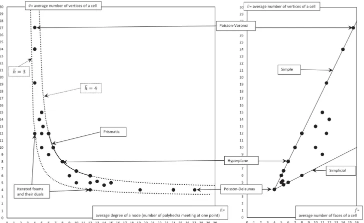
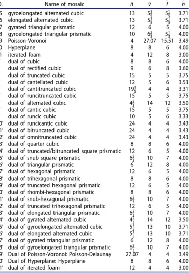
To provide the complete list of these 28 honeycombs has been a major result in discrete geometry. If these mosaics were spread out on the½n,vsymbolic plane, that would certainly imply that the associated values of the harmonic degreeh cover a very broad range. However, this is not the case: all values of h are in the range 3:31h4: In addition, we also computed the values of h associated with the 28 dual mosaics, hyperplane random mosaics, the Poisson- Voronoi and Poisson-Delaunay random mosaics and found that for the total of all the 60 mosaics the range is the same (cf. Table A1in the Appendix). The indicated narrow range for the harmonic degree implies that on the ½n,v symbolic plane the points corresponding to these mosaics appear to accumulate on a narrow strip (cf.Figure 1).

While we can not offer a full explanation of this phenomenon, we think that the concept of the harmonic degree may help to explain its essence. In particular, we introduce Conjecture 1. For any normal, face-to-face mosaic M in R^d, we havehðMÞ 2 ðd, 2^d1:

To build intuitive support for Conjecture 1 we will show inSection 3that the interval indicated in the Conjecture has indeed some significance: we demonstrate mosaics corresponding to the lower and upper endpoints (the former understood as a limit outside the interval) and we also prove

Theorem 2. For allh^?2 ðd, 2^d1, there is a normal, face-to- face mosaicMinR^d satisfyinghðMÞ ¼h^?:

Also, as a small step towards establishing the Conjecture, we prove

Proposition 1. For any normal, face-to-face mosaic M in R^d, we have hðMÞ ^dþ1₂ : Furthermore, if d¼3, thenhðMÞ ²⁸₁₃:

We provide the general formulae governing 3 D mosaics inSection 2. Next, we prove Theorems 1 and 2 inSection 3.

Section 4 discusses non-Euclidean mosaics and non-face-to- face mosaics ind¼2 and d¼3 dimensions. In Section 5we draw conclusions.

2. General formulae defining 3D mosaics

In [11], for any 0i,jdand for any random mosaicM in thed-dimensional Euclidean spaceR^d, the quantitynij is defined as the number of j-faces of a typical i-face of M if ji, and as the number of j-faces containing a typical i- face of M if j>i. Relations between these quantities are described in [11, Theorem 10.1.6] for the cased¼2, and in [11, Theorem 10.1.7] for the case d¼3. Here we use elementary, combinatorial arguments to show that these relations hold for any convex mosaic inR³:

(4)

Throughout this section, let Mbe a convex, face-to-face, normal mosaic in R^d: Then we may define nijðMÞ as the averagenumber ofj-faces contained in or containing a given i-face, ifjiorj>i, respectively. If it is clear which convex mosaic M we refer to, for brevity we may use the notation nij¼nijðMÞ: Here we assume that the average of any nij, for all values ofiandjexists.

Theorem 3. For any convex mosaic M in R³ satisfying the conditions in the previous paragraph, we have

nijðMÞ

¼

1 ðf2Þn

v þ2 ðf2Þn

v þn n

2 1 2ðvþf2Þn

ðf2Þnþ2v

2ðvþf2Þn ðf2Þnþ2v 2ðv2Þ

f þ2 2ðv2Þ

f þ2 1 2

v vþf2 f 1

2 66 66 66 66 66 4

3 77 77 77 77 77 5 ,

(2) wherev¼n30,f ¼n32 andn¼n03:

Proof. Clearly, nii ¼1 for i¼1, 2, 3, 4, and since each face belongs to exactly two cells, and each edge has exactly two endpoints, we have n23¼n10¼2: The formula n31¼ vþf 2 follows from applying Euler’s formula for each cell of M, and observing that then the same formula holds for the average numbers of faces, edges and vertices of a cell.

Let r be sufficiently large, and let Br be the Euclidean ball, centered at the origin o and with radius o. Let NvðrÞ,NeðrÞ,NfðrÞ andNcðrÞ denote the number of vertices, edges, faces and cells of MinBr, respectively.

Note that ifris sufficiently large, the sum of the numbers of edges of all faces in Br is approximately NfðrÞn21, and since almost all face in Brbelongs to exactly two cells inBr, and each edge of a given cell belongs to exactly two faces of the cell, we have that this quantity is approximately equal to NcðrÞn31: On the other hand, the sum of the numbers of faces the cells in Br have is approximately NcðrÞf 2NfðrÞ: More specifically, we have

f

2¼_r!1limNfðrÞ NcðrÞ¼n31

n21

, which readily yields thatn21¼n20¼^2ðvþf2Þ_f :

Note that the number of cell-vertex incidences in Br is approximately NvðrÞnNcðrÞv: Furthermore, for any incident cell-vertex pair C, v, the number of faces that contain the vertex and is contained in the cell is equal to the number of edges with the same property. Let us denote this common number by deg_CðvÞ, which then denotes the degree of the vertex v in the cell C. We compute the approximate value of the quantityQ¼P

CBr,v2Cdeg_CðvÞin two different ways.

On one hand, we have Q¼ X

CBr

2eðCÞ 2n31NcðrÞ,

Figure 1. The 28 uniform honeycombs, their duals, the hyperplane mosaics, the Poisson-Voronoi and Poisson-Delaunay mosaics, iterated foams and their duals (for details on the latter see Section 3.2) shown as black dots on the symbolic plane½n,v(left) and on the plane½f,v, wheref denotes the average number of faces of a cell of the mosaic (right). For detailed numerical data seeTable A1in the Appendix. Continuous curve on the left panel shows prismatic mosaics. Dotted lines represent theh¼3 andh¼4 curves, illustrating Conjecture 1. Continuous straight lines on the right panel correspond to simple and simplicial polyhedra.

(5)

where e(C) denotes the number of the edges of the cell C.

On the other hand, since any face belongs to exactly two cells, we also have

Q¼X

v2Br

X

CBr,^C像v

deg_CðvÞ 2n02NvðrÞ: More precisely, we have obtained that

n

v¼_r!1lim NcðRÞ NvðrÞ ¼n02

n31, which implies the expression for n02.

The value ofn01can be obtained from the application of Euler’s formula for the vertex figure at every node. Finally, the value of n12¼n13 can be obtained from the values of the other nijs like the value ofn20 ¼n21:

Remark 1. ByTheorem 3, it seems that many combinatorial properties of the convex mosaic Mare determined by three parameters, say by v, f, n. One may try to find upper and lower bounds for these values by observing that each entry in ½nij has a minimal value: e.g. n30,n32,n03,n014 and n12,n213: Nevertheless, solving these inequalities puts no restriction on the values of v, f, n, apart from the trivial inequalities n,v,f 4: It is worth noting that in contrast, for convex polyhedra (or, in other words, for convex spherical 2-dimensional mosaics, cf. Remark 8), the sharp inequalities ^v₂þ2f 2vþ4 [14, 15] are immediate con- sequences of the fact that each face of the polyhedron has at least 3 vertices, and each vertex belongs to at least 3 faces.

Remark 2. Note that if M is a convex mosaic inR³ and a convex mosaicM is its dual, then

nijðMÞ ¼n_ð3iÞð3jÞðMÞ, for all 0i,j3:

3. Proof of the theorems

3.1. Proof of Theorem 1 and the volumes of polar domains

Proof. First we show that in case of Euclidean mosaics (in arbitrary dimensions) the harmonic degree may be inter- preted as the averaged inverse sum of two angles linked by polarity, one of which is the internal vertex angle of a cell.

Consider a convex face-to-face mosaicMinR^d:For any cell CinMand any vertexpofC, letIðC,pÞ S^d1denote the set of unit vectors such that the rays in the direction of a vector in I(C,p) and starting atpcontain points ofCn fpg:Furthermore, letEðC,pÞ S^d1denote the set of outer unit normal vectors of C atp. Then, by definition, we have that E(C, p) is the polar ðIðC,pÞÞofI(C,p). Let us denote the spherical volumes ofE(C, p) andI(C, p) by XEðC,pÞandXIðC,pÞ, respectively, and let XE,XI define the average values of XEðC,pÞ and XIðC,pÞ, respectively, over all incident pairsCandp.

Note that for any cellC, the family of setsE(C,p), where p runs over the vertices of C, is clearly a spherical mosaic of S^d1, and thus, the total area of the members of this family is the surface area Sd1 of the sphere. The same statement

holds for the family of sets I(C, p), where C runs over the cells containing a given nodep.

Now, consider a large ball Bof space with radius r, and denote by Nc andNv the numbers of cells and nodes ofM in B, respectively. Then, for the number k(r) of incident pairs of cells and vertices inBwe have

kðrÞ NcvNvn: (3) The sums xI,xE of XIðC,pÞand XEðC,pÞ (over all pairs of cellsCand incident verticesp inB) may be written as:

x^I NvSd1

xE NcSd1, (4) so, for the averages XI¼limr!1ðxI=kÞ,XE¼ limr!1ðxE=kÞwe get

XIn¼XEv¼Sd1: (5) Thus, by (5) we have

X ¼XIþXE¼Sd1

v þSd1

n , (6)

implying that

hX ¼Sd1: (7)

Remark 3. Substituting the value ofSd1 into (7), we obtain that for planar mosaics h¼²_X^p, and for mosaics inR³h¼⁴_X^p:

Remark 4. Ifd¼2, then at each vertex we have XIðC,pÞ þ XEðC,pÞ ¼p, implying X ¼p and this, via equation (7) yieldsh¼2:

Remark 5. As we observed, for any node p and any cell C incident top, we have

X

fp:p2Cg

XEðC,pÞ ¼ X

fC:p2Cg

XIðC,pÞ ¼Sd1: While the equality

X

fC:p2Cg

XEðC,pÞ ¼Sd1

does not hold in general, it does hold in case of hyperplane mosaics.

Remark 6. Clearly, the inequalitiesv,n4 readily implyh 2, and by Theorem 1, X ¹₂Sd1: This inequality is also an immediate consequence of the well-known result of Gao, Hug and Schneider [6], stating that for any spherically convex setA of a given spherical volume, the volume of its polarAis maximal ifAis a spherical cap of the given spherical volume.

3.2. Proof ofTheorem 2 and the range of the harmonic degree

3.2.1. Mosaics with high harmonic degree:

hyperplane mosaics

IfMis generated by dissectingR^d withðd1Þ-dimensional hyperplanes then it is called a hyperplane mosaic [11]. An

(6)

elementary computation shows that the harmonic degree of a normal mosaic, generated by hyperplanes in general pos- ition, is

h¼2^ðd1Þ: (8) These mosaics appear to have the highest harmonic degree. They are certainly not the only mosaics with h¼ 2^d1, though. In d¼2 dimensions all convex mosaics have h¼2 and in d¼3 dimensions we have the continuum of prismatic mosaics withh¼4:

3.2.2. Mosaics with low harmonic degree: iterated foams and their duals

Here we define mosaics which appear to have extremely low harmonic degrees.

Consider a Euclidean mosaic M ¼ M0 with n0¼dþ1 as the average degree of nodes; we remark that such mosaics exist in all dimensions, we construct the dual of such a mosaic in the proof of Theorem 2. In addition, we assume that the edge lengths of the mosaic are uniformly bounded;

that is there are some 0<a<b such that the value of each such quantity is betweena andb, and we assume the same about the angles between any two faces ofM:

Note that since all d-dimensional convex polytopes with dþ1 vertices are simplices, the vertex figures of ‘almost all’ nodes of M are simplices. Now, for each node having a simplex as a vertex figure, replace the node with its vertex figure. More precisely, ifpis a node whose vertex figure is a simplex, define the cell Cp as the convex hull of the points of the edges starting at p, at the distance e>0 from p for some fixed value of e independent of p, and replace each cell C containingp with the closure ofCnCp: Then, if this process is carried out simultaneously at all nodes p, we obtain a convex, face-to-face mosaic M1, which, under our condition, is normal. Applying this procedure k times we obtain the convex, face-to-face, normal mosaicM_k:We will call the k! 1 limit of such a sequence a d-dimensional iterated foam, referring to the fact that in a physical foam in d¼2 andd¼3 dimensions we always haven¼dþ1:

Clearly, for all k1, we have nk¼nðMkÞ ¼dþ1:

Consider a sufficiently large region of space. Then the number of vertex-cell incident pairs in M is approximately NcvNvn¼Nvðdþ1Þ, where Nc andNv denote the numbers of the cells and the nodes of the mosaic in this region, respectively. An elementary computation yields that for the mosaic M1, this number is approximately Ncdvþ ðdþ 1ÞNv ðdþ1ÞNcv, and the number of cells of M1 in this region is about NcþNv1þ_dþ1^v

Nc: Thus, taking limit, we obtain that the average degree of a cell of M1 is

vðM1Þ ¼^ðdþ1Þ_dþ1þ²_v^v: Setting vk¼vðMkÞ, we similarly obtain the recursive formulavkþ1¼^ðdþ1Þ_dþ1þ²_v^v^k

k for all nonnegative integers k.

An elementary computation yields that jvkþ1dðdþ 1Þj ¼^ðdþ1Þj_dþ1þ^v^k^dðdþ1Þj_v_k ¹₂jvkdðdþ1Þj for all vkdþ1: This implies that for any initial value vdþ1, the sequence fvkg converges to dðdþ1Þ, and thus, the sequencefhðMkÞgconverges todðdþ1Þþðdþ1Þ^dðdþ1Þ² ¼d:

We note that the above procedure can be dualized. In this case, starting with a mosaic in which all cells are simplices, in each step we divide the cell into regions by taking the convex hulls of a given interior point of the cell with each facet of the cell. Lines 31 and 31⁰ of Table A1 in the Appendix summarize the main parameters of these iterated mosaics.

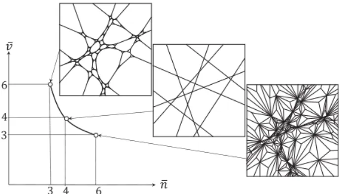
Remark 7. We note that for planar mosaics the iterating process (and also its dual), can be extended to any mosaic in a natural way, and after one iteration step the degree of every node (in case of its dual the degree of every cell) is equal to 3. This is illustrated in Figure 2where we iterate a (finite domain of a) hyperplane mosaic for k¼2 steps in both directions.

3.2.3. Proof ofTheorem 2

Let M be the standard cubic mosaic in R^d, whose vertices are the points of the integer lattice Z^d, and note that h¼ 2^d1: We define a new lattice M⁰ as the first barycentric subdivision ofM:In this lattice the centroid of each face of M is a vertex of M⁰, and cells correspond to flags of M, where a flag is a sequence F0F1F2:::Fd of faces ofM, with dimFi¼ifor all values ofi. In this case the cell associated to the flag is the convex hull of the centroids of theFis.

We compute the harmonic degree of M⁰:Note that since every cell ofM⁰ is a simplex, we havevðM⁰Þ ¼dþ1: First, observe that since any cell of M has 2d facets and by the fact the every face of a cube is a cube, choosing the faces of a flag in the order Fd,Fd1,:::,F0, we have that the number of flags belonging to any given cube in the mosaic is 2d ð2d2Þ ::: 2¼2^dd!: We note that the same quantity can be obtained if we choose the faces of a flag in the opposite order. In this approach first we choose a vertex of the cell, then we extend this point to an edge parallel to a chosen coordinate axis, which then can be extended to a 2-face choosing another coordinate axis. In this way the number of

Figure 2. Illustration of an iterated foam and its dual in d¼2 dimensions. We used the hyperplane mosaic (middle panel) as initial condition and ran k¼2 iterative steps both in the direction of iterated foams (upper panel) as well as their duals (lower panel). Note that in d¼2 dimensions these iterative steps change bothnandv, however, the harmonic degree remains constant ath¼ 2:Also note that in higher dimensions hyperplane mosaics may not be used as initial conditions for these iterations. Iterated foams and their duals in d¼3 dimensions are shown in the symbolic plane onFigure 1.

(7)

flags is equal to the product of the number of vertices (2^d), and the number of permutations of the d coordinate axes (d!).

Applying arguments similar to these two counting arguments, one may show that each i-face belongs to 2ⁱi!ðdiÞ! flags within one cell, and as each i-face belongs to 2^di cells, the total number of flags an i-face belongs to is 2^di!ðdiÞ!:

Furthermore, the proportion of the i-faces compared to the number of cells is d

i

: Thus, the average degree of a node in the barycentric subdivision of the cubic lattice is

nðM⁰Þ ¼

Pd

i¼02^di!ðdiÞ! d i Pd

i¼0 d

i

¼ ðdþ1Þ!,

implying

h⁰¼hðM⁰Þ ¼ðdþ1Þ!

1þd! , (9)

where an elementary computation yields that d^ðdþ1Þ!_1þd! <

dþ1 for alld1:

Case 1, h⁰¼^ðdþ1Þ!_1þd! h^?h¼2^d1: We construct a mosaic with harmonic degree h^?:To do it, we use four types of layers.

A first type layer is a translate of the part of the cubic lattice between the hyperplanes fxd ¼0g and fxd ¼1g: A second type layer is the same part of the subdivided cubic lattice M⁰: For the third type, we take the translates of a partial subdivision of the cubic lattice: each cube in the strip between fxd¼0g and fxd ¼1g is subdivided by the centroids of all faces apart from those in the hyperplane fxd ¼ 1g: The fourth type layers are the reflected copies of third type layers about the hyperplane fxd ¼0g:

The building bricks of the mosaic are strips S(k, l) of width kþlþ2, where k and l are positive integers. Here S(k, l) consisting of k first type, 1 fourth type,l second type and 1 third type layer in this consecutive order, where the layers are attached in a face-to-face way. Observe that if k and l are sufficiently large, then the harmonic degree of a stripS(k, l) is approximately_kþl^k hþ_kþl^l h⁰:

Since h⁰h^?h, there is some 0k1 such that h^?¼khþ ð1kÞh⁰: Let fðkm,lmÞg be a sequence of pairs of positive integers such that kmþlm! 1, and_k^k^m

mþlm!k:

We define the mosaic M^? as follows. Consider a strip S1¼Sðk1,l1Þ: Attach two copies of Sðk2,l2Þ to the two bounding hyperplanes of S1 in a face-to-face way, to obtain S2 as the union of these three strips. Then S3 is constructed by attaching two copies of Sðk3,l3Þ to S2 in a face-to-face way. Continuing this procedure, we obtain the mosaic M^? as the limit of the strip Sm, where m! 1: Then the harmonic index of M^? ish^?:

Case 2,d<h^?<h⁰:Observe that in the subdivided cubic mosaic M⁰ defined above, every cell is a simplex. Thus, we may apply the dual of the algorithm discussed in Subsection 3.2.2, namely in each step we divide each cell C into dþ1 new cells by taking the convex hulls of a given interior point

of C and the facets of C. Let us denote by Mk and hk the mosaic obtained by k subsequent applications of this procedure, and its harmonic degree, respectively. Then the sequencefhkgtends to d, and thus, there is a smallest value ofk such thath^? is in the interval ½hkþ1,hk:To construct a suitable mosaicM^? with harmonic degreeh^?, we follow the idea of the proof in Case 1, and divide only a part of the cells ofMkinto new cells.

3.2.4. Proof of Proposition 1

The first part of the proposition follows from the trivial esti- mates v,ndþ1: To prove the second part, we need a lemma. We note that the minimum number of tetrahedra such that each convex polyhedron with k vertices can be decomposed into is not known. This fact and the idea of the proof of Lemma 1 can be found in [4].

Lemma 1. Any convex polyhedron P in R³ with v vertices can be decomposed into at most2v7tetrahedra.

Proof. Let the faces of P beG1,:::,Gf, and let fi denote the number of edges of Gi. Then Pf

i¼1fi¼2e¼2vþ2f4, whereeis the number of edges ofP.

Letpbe any vertex of P. Let us triangulate each face ofP containing p by the diagonals starting at p, and all other faces of P by the diagonals starting at an arbitrary vertex of the face. Then the number of all triangles isPf

i¼1ðfi2Þ ¼ 2vþ2f 42f ¼2v4: Since each face contains at least one triangle, and each vertex belongs to at least three faces, the numbermof triangles in the faces not containingp is at most m2v7: Now, if these triangles are T1,T2,:::,Tm, then the tetrahedra convðfpg [TiÞ,i¼1, 2,:::,m is a

required decomposition ofP. w

Consider a mosaic M in R³, and a sufficiently large region. LetNcandNvdenote the numbers of cells and nodes of Min this region. For any cell Ci, let vi denote the number of vertices ofCi. Then the number of cell-vertex incidences in this regions is approximatelyP

iviNcvNvn:

ByLemma 1, these cells can be decomposed into at most P

ið2vi7Þ 2Ncv7Nc tetrahedra. It is well known that the sum of the internal angles of any tetrahedron is greater than 0 and less than 2p [5]. Thus, the sum of all the internal angles of the cells is at most 4pNcv14pNc: On the other hand, this sum is approximately equal to the product of the number of nodes and the total angle of a sphere; that is 4pNv: Thus, apart from a negligible error term, we have 4pNcvn4pNcv14pNc: Taking a limit, we obtain that 2vn2v7, implying that n₂_v7²^v : Since n4 clearly holds, we have that

nmax

4, 2v

2v7 : (10)

It is an elementary computation to check that 4₂_v7²^v if and only ifv¹⁴₃ :Since for any fixed value of n,h is minimal at the minimal value ofvit follows that under the condition that v¹⁴₃, we have h²⁸₁₃: Furthermore, if

(8)

4v¹⁴₃, then h¼₂_v5²^v , which is minimal ifv¼¹⁴₃ , and thus,h²⁸₁₃also in this case.

4. Non-Euclidean and non face-to-face mosaics 4.1. Non-Euclidean mosaics

Mosaics, convex mosaics, and all notions described in Subsection 1.1, excluding the notions of average degrees of cells and vertices, can be defined in a natural way for spherical and hyperbolic spaces as well. For spherical space, this includes average degrees as well; because of the compactness of the space it is even possible to avoid the usual limit argument applied to compute these values inR^d:

On the other hand, defining average values in hyperbolic space seems problematic. Indeed, it is well known that under rather loose restrictions, in a packing of congruent balls in H^d, the number of balls intersecting the boundary of a hyperbolic ball Bof large radius is not negligible compared to the number of balls contained inB. This phenomenon is explored in more details, for instance, in [3], and can be generalized for the numbers of cells of a normal mosaic in a natural way.

A straightforward solution to this problem is to examine only regular mosaics, in which the degree of every cell, and the degree of every vertex is equal, which offers a natural definition for n and v: We do this in Subsection 4.1.1. To circumvent this problem in a more general way, we use the geometric interpretation of harmonic degree for mosaics in R^d, appearing in Subsection 3.1; this interpretation, in particular, provided a different proof of the fact that harmonic degree is 2 for every planar Euclidean mosaic.

In Subsection 4.1.2 we generalize this geometric interpretation for mosaics inS² andH², and show that for spherical mosaics it coincides with the original definition of harmonic degree. Finally, we show that this value is less than 2 for any spherical mosaic, and it is at least 2 for any hyperbolic mosaic, using any reasonable interpretation of average.

4.1.1. Non-Euclidean regular honeycombs inS^d,H^d for d¼2, 3

Here we show that in d¼2 dimensions, Euclidean mosaics separate regular spherical mosaics from regular hyperbolic mosaics on the½n,vsymbolic plane.

While Plato’s original idea of filling the Euclidean space with regular solids proved to be incorrect, if we relax the condition that the embedding space has no curvature then all Platonic solids may fill space by what we call a regular honeycomb. We briefly review these mosaics to show how they are represented in our notation and how their harmonic degrees are spread.

Let Mbe a honeycomb in a space of constant curvature of dimension d. A sequence F0F1:::Fd, where Fi is an i-dimensional face of M, is called a flag of M (cf. the proof of Theorem 2). We say that M is regular, if for any two flags of M there is an element of the symmetry group ofMthat maps one of them into the other one. In particular, ifMis a regular planar mosaic, then the cells of Mare

congruent regular p-gons, and at each node, an equal q number of edges meet at equal angles. In this case fp,qgis called the Schl€afli symbol of M: It is well known that up to congruence, for any values p,q3, there is a unique regular mosaic with Schl€afli symbol {p, q} (cf. [12]). This mosaic if spherical if p¼3 and q¼3, 4, 5 or if q¼3 and p¼3, 4, 5, Euclidean if fp,qg ¼ f3, 6g,f4, 4g,f6, 3g, and hyperbolic otherwise. We note that the five regular spherical honeycombs correspond to the five Platonic polyhedra. The Schl€afli symbol of a higher dimensional mosaic can be defined recursively: it is fp1,p2,:::,pdgif the Schl€afli symbol of its cells are fp1,p2,:::,pd1g(which must correspond to a regular spherical mosaic), and the intersection of M with any sufficiently small sphere centered at a node ofM is the regular spherical mosaicfp2,p3,:::,pdg:

Ind¼2 dimensions the h¼2 curve defines a partition of theZ² grid on the½n,v symbolic plane with the constraints

n,v3:For a regular mosaic with Schl€afli symbolfp,qg, set

v¼p,n¼q, or equivalently, h¼_pþq^pq : Then an elementary computation (determining the sign of the quantity ¹_pþ¹_q¹₂ for all integersp,q3) shows that grid points on theh¼2 line correspond to regular Euclidean mosaics, grid points with h<2 correspond to regular spherical mosaics and grid points withh>2 correspond to regular hyperbolic mosaics.

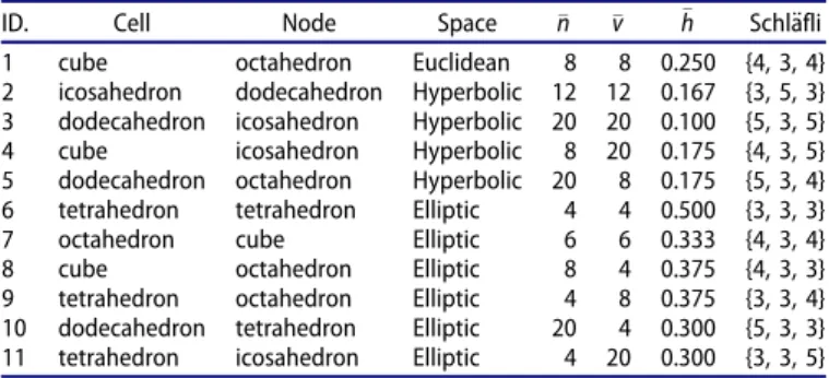
In d¼3 dimensions the h¼4 curve defines a partition of theZ² grid on the½n,vsymbolic plane in a similar sense, although here only a finite number of grid points correspond to regular mosaics. We summarize these inTable 1.

As we can observe, the harmonic degree h of a mosaic appears to carry information both on the dimension and the curvature of the embedding space: h¼constant curves separate convex mosaics embedded in spaces with the same curvature sign but different dimension and vice versa, they also separate regular mosaics embedded in spaces with the same dimension but different sign of curvature. Knowing one of those parameters seems to permit us to obtain the other, based on the mosaic’s harmonic degree.

4.1.2. Non-Euclidean general face-to-face mosaics on S² andH²

Our goal is to extend the geometric interpretation of the harmonic degree to convex face-to-face mosaics on S² and H²:First we describe how the duals of spherical mosaics can be constructed. To do this, first we compute the harmonic degree of spherical mosaics directly.

Table 1. Regular honeycombs in d¼3 dimensions.

ID. Cell Node Space n v h Schl€afli

1 cube octahedron Euclidean 8 8 0.250 {4, 3, 4}

2 icosahedron dodecahedron Hyperbolic 12 12 0.167 {3, 5, 3}

3 dodecahedron icosahedron Hyperbolic 20 20 0.100 {5, 3, 5}

4 cube icosahedron Hyperbolic 8 20 0.175 {4, 3, 5}

5 dodecahedron octahedron Hyperbolic 20 8 0.175 {5, 3, 4}

6 tetrahedron tetrahedron Elliptic 4 4 0.500 {3, 3, 3}

7 octahedron cube Elliptic 6 6 0.333 {4, 3, 4}

8 cube octahedron Elliptic 8 4 0.375 {4, 3, 3}

9 tetrahedron octahedron Elliptic 4 8 0.375 {3, 3, 4}

10 dodecahedron tetrahedron Elliptic 20 4 0.300 {5, 3, 3}

11 tetrahedron icosahedron Elliptic 4 20 0.300 {3, 3, 5}

(9)

Remark 8. Clearly, projecting a convex polyhedron P from an interior point to a sphere concentric to this point yields a spherical mosaic. Furthermore, in a spherical mosaic any two cells intersect in one edge, one vertex or they are disjoint. Using these properties it is easy to show that the edge graph of any spherical mosaic is 3-connected and planar;

such an argument can be found, e.g. in the proof of [1, Claim 9.4]. By a famous theorem of Steinitz [15], every 3- connected planar graph is the edge graph of a convex polyhedron. Thus, up to combinatorial equivalence, we may regard a spherical mosaic as the central projection on S² of a convex polyhedron P containing the origin in its interior.

This representation permits us to define the dual of a spherical mosaic associated to P as the mosaic associated to its polar convex polyhedronP:

In two dimensions, spherical mosaics may be characterized by the angle excess associated with their cells which is equal to the solid angle subtended by the cell or, alterna- tively, the spherical area of the cell. Let M be a convex mosaic on S² with Nv nodes and Nc cells. Since Mis a til- ing of S², the average area of a cell is XC¼^4p_N

c: Similarly, the average area of a cell in the dual mosaic isXN ¼⁴_N^p_v: Definition 3. For any spherical mosaic M, we call the quantity lðMÞ ¼_p¹_X^X^C^X^N

CþXN theharmonic angle excessof M: Proposition 2. The harmonic degree of any convex, face-to- face mosaic MonS² is

hðMÞ ¼2lðMÞ: (11)

Proof . Let Nc and Nv denote the numbers of cells and nodes ofM, and letvandn denote the average degree of a cell and a node, respectively. Then the number of adjacent pairs of cells and nodes ofMis equal to

vNc¼nNv: (12)

Let aij denote the angle of the cell Ci at the vertex vj if they are adjacent, and let aij¼0 otherwise. We compute the sum P

i,^jaij in two different ways. First, note thatP

i,^jaij¼ P

j

P

iaij¼2pNv: On the other hand, the area of any cell Ci is equal to the angle sufficit of Ci, or more specifically, areaðCiÞ ¼P

jaij ðdegðCiÞ 2Þp, where degðCiÞ is the number of vertices of C_i (see Subsection 1.1). Since P

iareaðC_iÞ ¼areaðS²Þ ¼4p and P

idegðC_iÞ ¼vC, it follows that P

i,^jaij¼4pþvNcp2Ncp: This implies the equality

2Nv¼vNc2Ncþ4: (13) Now, (11) follows from (12, 13) and the equation l¼

4

NvþNc(which follows from Definition 3). w

Corollary 1. The harmonic degree of any face-to-face convex mosaicMofS²is

hðMÞ<2:

While it does not seem feasible to extend the definition of h for mosaics in H² in a straightforward way, the

geometric interpretation of this quantity in Subsection 4 permits us to find a variant ofCorollary 1also in this case.

Let M be a convex face-to-face mosaic in any of the planes R²,S² or H²: Let C be a cell of M with v vertices.

Letpj,j¼1, 2,:::,vbe the vertices of C, and fix an arbitrary point q2 int C: Let Lj denote the sideline of C passing through the vertices pj and pjþ1, and let Rj denote the ray starting atqand intersectingLjin a right angle. The convex- ity of C implies that the rays R1,R2,:::,Rv are in this cyclic order aroundq. Let XEðC,pjÞ denote the angle of the angu- lar region which is bounded byRj1[Rjand whose interior is disjoint from all the rays Rj⁰: Furthermore, let XIðC,pjÞ denote the interior angle of C at pj. Now we define the quantity

XðCÞ ¼ Pv

j¼1ðXEðC,pjÞ þXIðC,pjÞÞ

v ¼2pþKðCÞ

v ,

whereKðCÞis the sum of the interior angles ofC.

Observe that if M is a Euclidean mosaic, then the weighted average value ofXðCÞ, with the weight equal tov, over the family of all cells ofMcoincides with X:

Next, assume that M is a spherical mosaic. Let the cells of M beCi, i¼1, 2,:::,Nc, and let Nv and Ne be the number of nodes and edges of the mosaic, respectively. If the degree of Ci is vi, then PNc

i¼1vi¼2Ne, and by Euler’s formula, NvþNc¼Neþ2, yielding l¼_N ⁴

cþNv¼_N⁴

eþ2: Furthermore, for all values of i, the area formula for spherical polygons yields thatKðCiÞ ¼ ðvi2ÞpþareaðCiÞ:Thus, XðCiÞ ¼^vⁱ^pþareaðC_v ⁱ^Þ

i : Since the total area of all cells is 4p, this implies

X ¼ PNc

i¼1XðCiÞvi

PNc

i¼1vi

¼pPNc

i¼1viþPNc

i¼1areaðCiÞ 2Ne

¼Nepþ2p Ne

¼ 2p 2l:

We have shown that for face-to-face, convex mosaics on S², we have h¼2l, (cf. (11)). Thus, for these mosaics we have h¼2pX, extending Theorem 1 for 2-dimensional spherical mosaics.

Finally, consider the case thatM is a hyperbolic mosaic.

Let Ci,i¼1, 2,::: denote the cells of M, and let vi denote the degree of Ci. As in the spherical case, by the area formula for hyperbolic polygons, we have that XðCiÞ ¼ p^areaðC_v ⁱ^Þ

i <p for all values ofi. For any nonnegative func- tion f :N!R, we may define the harmonic degree of M with respect to fas

hf ¼ lim

k!1

2pPk i¼1fðiÞvi

Pk

i¼1fðiÞviXðCiÞ,

where the inequalities XðCiÞ<p,i2N imply hf 2: Note that since any measure on a countable set is atomic, the above formula exhausts all reasonable possibilities for defining harmonic degree.

(10)

4.2. Non face-to-face mosaics onR² andS²

Conjecture 1 formulates the hypothesis that the harmonic degree of d-dimensional Euclidean face-to-face mosaics is confined to the rangeðd, 2^d1: In the current subsection we would like to point out that in case of non face-to-face mosaics this range may be much broader. According to the convention introduced in Subsection 1.1, the degree of a node is equal to the number of vertices coinciding at that node, both for face-to-face and non face-to-face convex mosaics.

In d¼2 dimensions we already stated that for face-to- face mosaics we have h¼2 [11, Theorem 10.1.6], which is equivalent to

n¼ 2v

v2: (14)

If we admit non face-to-face mosaics and we sum the internal angles over all cells and also sum the same angles as nodal angles over all nodes then (14) generalizes to

n¼ 2v

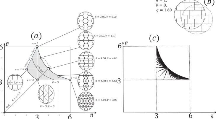
vp1, (15) wherep is the proportion of the regular nodes in the family of all nodes, where we call a node regular if it is the vertex of every cell it belongs to. As we can see, in 2 dimensions convex mosaics have two free parameters and they form a compact, 2D subset of the½n,v symbolic plane as illustrated in Figure 3. By computing the harmonic degree h over the admissible domain marked on Figure 3(a) we find that

1:33h2 which indicates that non face-to-face mosaics may admit lower harmonic degrees than face-to-face mosaics. Figure (3) (b) shows an example of a non face-to- face mosaic ind¼3 constructed as alternated, shifted layers of a brick-wall-type planar mosaic. At every node just 2 vertices meet so we haven¼2 and each cell is a cuboid yielding v¼8: This results in a valueh¼1:6 which is certainly below the maximal value ofh¼2 for planar mosaics.

Remark 9. Using the proof of Proposition 2, the generaliza- tion of formula (15) to 2D spherical mosaics is straightforward:

v¼ ð2lÞn

nþl1p: (16)

5. Summary

In this paper we proposed to represent mosaics in the½n,v symbolic plane of average nodal and cell degrees and we introduced the harmonic degreeh, constant values of which appear as curves in this space. We pointed out that these curves appear to have special significance: in d¼2 dimensions all convex, face-to-face mosaics appear as points of the h¼2 curve and a compact domain can be associated to non face-to-face mosaics. We showed that in case of 2D spherical mosaics h differs only in a constant from the suitably averaged angle excess and this explains why points associated

Figure 3. (a) Symbolic plane for planar mosaics. The p¼1 line corresponds to face-to-face mosaics. Gray shaded area marks the descriptors of all admissible mosaics in the plane. (b) Example of a special 3D mosaic withh<2:Solid line: odd layer, dotted line, even layer. Both layers correspond to the planar mosaic in panel (a) atðn,vÞ ¼ ð2, 4Þ:(c) Parameter plane for spherical mosaics in d¼2 dimensions. All mosaics shown withNcþNv200, Ncdenoting the number of cells, Nvdenoting the number of nodes. Mosaics on thev¼3 andn¼3 lines correspond to simple and simplicial polyhedra, respectively. Observe how mosaics accumulate on the line corresponding to face-to-face Euclidean mosaics.