Interest premium and economic growth: the case of CEE

Interest premium and economic growth: the case of CEE

Dániel Baksa^∗ István Kónya^† April, 2017

Abstract

This paper views the growth and convergence process of the four Visegrad economies - the Czech Republic, Hungary, Poland and Slovakia - through the lens of the open econ- omy, stochastic neoclassical growth model. We use a unified framework to understand both the long-run convergence path and fluctuations around it. Our empirical exercise highlights both the role of initial conditions such as indebtedness and capital intensity, and random shocks in the growth process. In particular, we explore the importance of the external inter- est rate premium, and its role in driving investment and the trade balance.

Keywords: stochastic growth, technology shocks, interest premium, small open econ- omy, Bayesian estimation.

JEL: E13, O11, O41, O47

1 Introduction

After the collapse of the socialist system and the initial transition phase the four Visegrad economies - the Czech Republic, Hungary, Poland and Slovakia - has experienced a long period of robust growth. Until 2008, all countries have closed the at least some of the initial gap in 1995 relative to the advanced EU countries. Part of this growth was financed by foreign investment, lead- ing to persistent deficits in the trade balance and to increasing degrees of external indebtedness.

The convergence process has partly continued after the global financial crisis of 2009, although it slowed down markedly in the Czech Republic and Hungary. The crisis also led to a drastic adjustment in external positions, with substantial heterogeneity among the countries.

∗Central European University and Center for Economic and Regional Studies

†Center for Economic and Regional Studies and Central European University

Our goal in this paper is to examine the growth and convergence process of the Visegrad countries through the lens of the stochastic neoclassical growth model. In this we follow Aguiar and Gopinath (2007) and García-Cicco, Pancrazi and Uribe (2010), who estimate similar models for Latin-American countries (Mexico and Argentina). While the first article aims to identify transitory and permanent productivity shocks only, the second paper also allows for shocks to the foreign interest premium. In fact, a key question in this literature is to estimate the extent to which changes in external financial conditions - as captured by the interest rate - are responsible for fluctuations in the growth rate of emerging economies, relative to persistent shocks to growth prospects.

The literature has identified two main shocks that drove stochastic growth in small, open economies like the Visegrad countries. Aguiar and Gopinath (2007) compare Mexico and Canada, and conclude that in the former shocks to trend productivity growth are more important than in the latter. The main reason is that in emerging economies, like Mexico, the trade balance is counter-cyclical. Transitory TFP shocks imply a pro-cyclical trade balance, since households want to save part of the temporary windfall gains. Permanent and lasting trend shocks, on the other hand, imply improving growth performance for a while, leading to increases in current and future permanent income. In that case, households want to consume some of the future gains now, which implies a trade deficit.

García-Cicco, Pancrazi and Uribe (2010) criticize Aguiar and Gopinath (2007) for ignoring the role of financial shocks. In particular, they argue that external financing conditions - which can be taken as exogenous for small, open emerging countries - are important growth determi- nants. They estimate a financial frictions augmented RBC model on a century of Argentine data, and conclude that interest premium shocks are more important than trend productivity shocks.

Increases in interest premia induce recessions and improve the trade balance at the same time, thus they can also explain the counter-cyclicality of the latter. Moreover, in the absence of fi- nancial frictions the trade balance is a random walk, which is at odds with the data in emerging economies.

Other papers have also followed up on the technology vs. interest premium debate. Naoussi and Tripier (2013) and Guerron-Quintana (2013) showed that a common trend productivity com- ponent better explains medium-term GDP growth volatility in African countries than financial shocks. In contrast, Tastan (2013) finds that in Turkey financial shocks are more important. Many

papers try to understand the role of financial intermediation more deeply. Zhao (2013) builds a model where agents face liquidity constraints, and it is the changes in liquidity that lead to fluc- tuations in the risk premium. Minetti and Peng (2013) assumes asymmetric information between domestic and foreign creditors, which becomes effective when income prospects worsen. This leads to a large response in external financing, which increases country risk and the effective foreign interest rate.

We make a number of contributions to this literature in our paper. First, we extend the analy- sis of stochastic growth to a new set of countries. We believe that the four Visegrad countries are a good laboratory for the neoclassical model. They are emerging economies, which are highly open both to international trade and external finance. Their performance, as indicated earlier, is broadly in line with the predictions of the neoclassical model, where convergence is driven by improvements in total factor productivity (TFP) and capital accumulation. Openness allows countries to finance some of their additional investment and consumption from abroad, which is in line with the evidence. Also, after the introduction of market reforms in the early 1990s, the Visegrad economies have reasonably similar institutions to the advanced market economies of Western Europe, the natural reference group.

The Visegrad countries have similar economies, which allows us to estimate the exogenous driving forces of economic growth in a panel. While the time series are short, using a panel of four countries gives us degrees of freedom to identify the underlying shock processes. On the other hand, initial conditions differ significantly, including the initial levels of indebtedness and capital intensity. There is also substantial heterogeneity in the economic performance of the four countries, which we partly attribute to the observable initial differences, and to unobservable differences in idiosyncratic shocks.

Second, using a panel we can separate (“global”) shocks that affect all countries from (“local”) shocks that are specific to a country. An interesting question concerns the magnitude of these two components, both for productivity shocks and for interest rate developments. Especially for the latter we might expect global shocks to dominate, since we are studying small open economies.

On the other hand, the external vulnerability of the four countries differs significantly, thus we may find that country-specific “extra” premium shocks will be found, especially for the most exposed economy, Hungary.

Third, we use the same model to separate the deterministic trend (“convergence”) from the

stochastic fluctuations (“cycle”). This is an appealing alternative to using a statistical filter, since it utilizes prior information embedded in the convergence model. As we discussed above, we think the overall growth process of the Visegrad countries is well described by the neoclassical model, thus we can use it to predict the convergence paths in the absence of stochastic disturbances.

We proceed in two steps. After setting up the model, we first ignore the shocks, and given initial conditions - calibrated from national accounts data in 1995 - we simulate the nonlinear deterministic model. We then take the simulated paths as the “trend” components, and subtract them from the empirical time series to arrive at the “cyclical” component. Then we use the log- linearized version of the full, stochastic model and estimate the shock processes on the stationary variables.

Our result show that the neoclassical growth model - once augmented with a few real rigidi- ties - does a good job in capturing key aspects of the 1995-2015 developments in the Visegrad countries. Given the evolution of total factor productivity that we back out from the data, de- terministic convergence simulations provide a good fit for the overall paths of consumption, investment, the trade balance and employment.

Decomposing the fluctuations around the predicted growth paths, we find that interest pre- mium shocks were mostly responsible for fluctuations in the composition of aggregate expen- diture. In particular, premium shocks redirect spending between domestic absorption and net exports. This effect is particularly strong in heavily indebted Hungary, which was most exposed to external financial developments. The role of trend shocks is less clear-cut, but they were im- portant during particular episodes such as the early 2000s in Poland.

For the three key shocks - technology, trend growth and interest premium - we allow local and

“global” (common) innovations. Since the four countries are highly integrated into the European economy, we expect common components to drive at least some of the movements in these shocks. We find clear evidence for this in case of the premium shocks, especially during the run-up to joining the European Union in 2004. In all four countries, the substantial decline in the estimated interest premium was mostly due to the global component. Interestingly, this is not the case during the financial crisis of 2008-2009. This may partly be due to the fact that global financial market disturbances proved short lived, and we use annual data in our estimation. Also, and more importantly, there was substantial heterogeneity among the Visegrad countries at the start of the crisis. Hungary was most vulnerable, while the Czech Republic and Slovakia were

the least exposed. This heterogeneity in initial conditions and in subsequent developments is translated into local components by our linear estimation method.¹

The paper proceeds as follows. In Section 2, we describe the stochastic growth model. In Section 3, we use the model to simulate deterministic convergence paths, given initial conditions.

In Section 4, we estimate the stochastic version of the model to explain deviations from the predicted convergence paths. Finally, in Section 5 we conclude and discussed future avenues for research.

2 The model

We use a somewhat modified version of the stochastic, neoclassical growth model described in Gracía-Cicco, Pancrazi and Uribe (2010). This is a one-sector, small open economy, where pro- duction is divided among household consumption (C), capital investment (I), net exports (T B).

Production requires labor (h) and capital (K). Final good and factor markets are competitive, with flexible prices. The engine of growth is exogenous improvements in productivity, which process we specify later. For simplicity, and given the demographics of the Visegrad countries, we assume that there is no population growth.

It is well known that aggregate variables are more persistent than the basic neoclassical model predicts, even at the annual frequency (Christiano, Eichenbaum and Evans, 2005). In our case, this is an important issue, since the convergence simulations start at an arbitrary initial condi- tion, determined by data availability (typically 1995) and heavily influenced by the exact timing of economic transition in each country. For this reason we add a few real rigidities to the ba- sic model, which capture the slow adjustment of the main macro variables. These are external habits in consumption, investment adjustment costs, and employment adjustment costs. The latter could be modeled explicitly as search frictions, but since our goal is not to understand unemployment, we opt for a simple specification.

1Benczúr and Kónya (2016) provide an alternative framework, where a common shock may be able to explain the different experience of countries with different initial condition. Their setup is highly non-linear, but deterministic, hence we cannot use it in our stochastic approach.

2.1 Households

The representative household solves the following problem:

E0

∞

X

t=0

β^t

log Ct−χC¯t−1

− θ_t 1 +ηh^1+η_t

s.t. Ct+Dt=Wtht+Dt+1

R_t + Πt+Tt,

whereDt+1 is foreign debt carried into the next period, Rt is the gross interest rate on debt, andT_tis government spending financed by lump-sum taxes.²Households earn wages (W), and profits (Π) from the representative firm that they own. Note that consumption is subject to external habit formation.

There are three structural shocks that affect household decisions. First, we take government spending to be exogenous and random:

logT_t= (1−ρ_τ) log ¯T+ρ_τlogTt−1+ν_t^τ.

Second, the interest rate on foreign bonds is subject to exogenous disturbances. The interest rate also has an endogenous component, which depends on the external indebtedness of the economy (Schmitt-Grohé and Uribe, 2003):

R_t= ¯R+ψ

e^Dt/Yt−dy−1

+e^rt −1,

where

^r_t =ρr^r_t−1+ν_t^r.

Finally, labor supply - or more broadly, the labor market - is influenced by an exogenous termθ_t, given as:

logθt= (1−ρ_h) log ¯θ+ρ_hlogθt−1+ν_t^h

2We assume that government consumption is purely wasteful. Equivalently , we could include it in the utility function in an additively separable form.

The first-order conditions of the problem are given as follows:

1 Ct−χC¯t−1

= Λ_t

θh^η_t = Λ_tW_t Λt=βRtEtΛt+1,

whereΛ_tis the Lagrange multiplier associated with the budget constraint.

2.2 Firms

The problem of the representative firm is as follows:

maxEt

∞

X

t=0

β^tΛt

Λ₀

"

AtK_t^α(Xtht)^1−α−It− 1 +υ 2

ht

ht−1

−1 2!

Wtht

#

s.t. Kt+1 = (1−δ)Kt+

"

1−φ 2

I_t It−1

−g 2#

It

Firms own the capital stock, and accumulate it through investment, subject to an adjustment cost. The first order conditions of firms are as follows:

(1−α)Y_t ht

=W_t

"

1 +υ 2

h_t ht−1

−1 2

+ν h_t

ht−1

−1 h_t

ht−1

#

−υβEtWt+1

h_t+1 ht

2 h_t+1

ht

−1 Λ_t+1

Λt

Qt=βEt

αYt+1

K_t+1 + (1−δ)Qt+1

Λt+1

Λ_t 1−Q_t+φ

2 It

It−1

−g_t 2

Q_t=βφEt

It+1

I_t −g_t It+1

I_t 2

Λt+1

Λ_t Q_t+1

−φ I_t

It−1

−g_t I_t

It−1

Q_t

Productivity is stochastic, with two components as in Aguiar and Gopinath (2007). The vari- ableXtrepresent the trend component, which evolves according to the following process:

X_t Xt−1

=g_t

logg_t= (1−ρ_g) log ¯g+ρ_gloggt−1+ν_t^g.

This means that productivity is subject to trend shocks, in addition to the standard, transitory productivity shock:

a_t=ρ_aat−1+ν_t^a.

2.3 Equilibrium

Combining the household and firm first-order conditions, and writing down the aggregate re- source constraint, the evolution of the model economy is given by the following set of equations:

Λt= 1 C_t−χC¯t−1

(1−α)Yt

h_t =Wt

"

1 +υ 2

ht

ht−1

−1 2

+ν ht

ht−1

−1 ht

ht−1

#

−υβEtWt+1

ht+1

h_t 2

ht+1

h_t −1 Λt+1

Λ_t W_tΛ_t=θh^η_t

1 =βRt

Λt+1

Λ_t Q_t=βEt

αY_t+1

K_t+1 + (1−δ)Q_t+1 Λ_t+1

Λ_t 1−Q_t+φ

2 I_t

It−1

−g_t 2

Q_t=βφEt

I_t+1 It

−g_t I_t+1 It

2Λ_t+1 Λt

Q_t+1

−φ It

It−1

−gt

It

It−1

Qt

Y_t=C_t+I_t+T_t+D_t−D_t+1 R_t Kt+1 = (1−δ)Kt+

"

1−φ 2

I_t It−1

−gt

2# It

Yt=AtX_t^1−αK_t^αh^α_t R_t= ¯R+ψ

e^Dt+1/Yt−dy−1

+ e^rt −1

The stochastic processes for the structural shocks were defined above.

The system is not stationary, since productivity has a stochastic trend. We introduce variables in effective form, that are constant in the deterministic steady state: ct = Ct/Xt,it = It/Xt, y_t=Y_t/X_t,k_t+1 =K_t+1/X_t,d_t+1=D_t+1/X_t, andλ_t=X_tΛ_t. Using these new variables, the

equilibrium system is given as:

1 c_t−(χ/g_t)ct−1

=λ_t≡Λ_tX_t θh^η_t =w_tλ_t

(1−α) yt

h_t =βυEtwt+1

ht+1

h_t 2

ht+1

h_t −1 λt+1

λ_t

−w_t

"

1 +υ 2

h_t ht−1

−1 2

+ν h_t

ht−1

−1 h_t

ht−1

# (1) 1 =βRtEt

1 gt+1

λt+1

λt

Q_t=βEt

1 g_t+1

αg_t+1y_t+1

k_t+1 + (1−δ)Q_t+1 λ_t+1

λ_t (2) 1−Q_t+φg_t²

2 i_t

it−1

−1 2

Q_t=βφEtg_t+1² i_t+1

it

−1 i_t+1 it

2 λ_t+1 λt

Q_t+1

−φg_t² it

it−1

−1 it

it−1

Qt (3)

y_t=c_t+i_t+ξ_t+d_t

g_t − d_t+1 R_t tbt= dt

gt

−dt+1

Rt

kt+1= 1−δ gt

kt+

"

1− φg_t² 2

it

it−1

−1 2#

it

y_t=A_t k_t

g_t α

h^1−α_t Rt= ¯R+ψ

e^dt+1/yt−dy−1

+ e^rt −1

3 The long-run

To estimate the system, we follow the two-step procedure outlined in the Introduction. First, we ignore the stochastic shocks, and investigate the convergence properties of the model. For this purpose, we simulate the non-linear system of difference equations in (2) and fit the determin- istic model on our appropriately transformed data. Then we use the simulated time series, and interpret data deviations from the deterministic convergence path as driven by the stochastic shocks. We thus use the model both for detrending the data, and later to estimate the stochastic shocks. This way we can explicitly take into account that at least some of the growth features in the data are due to the fact that the Visegrad countries are converging towards a steady state in

the sample period.

3.1 Data

Most of our dataset comes from Eurostat, and includes chain-linked real series for GDP, con- sumption, investment, exports and imports, and total hours. The sample period is 1995-2015. For GDP components, we use shares, i.e.C_t/Y_t,I_t/Y_tandT B_t/Y_t. Without loss of generality, total hours are normalized such that they equal 1 for Germany in 1995. These variables are stationary, and can be used directly in the model simulations. We describe the normalization of GDP per capita below.

To simulate the model, we need initial conditions for the state variables. For initial debt we use the net foreign asset position of each country (relative to GDP), downloaded from central banks of the respective countries. To calculate initial capital and productivity levels, we use a standard development accounting exercise. First, we calculate capital stocks using the Perpetual Inventory Method. We assume that Germany is in its steady state in 1995, while for the Visegrad countries we postulate an initial capital-output ratio that is 75% of the country specific steady state value. This implies that part of growth in the sample period was driven by capital accumu- lation. Our choice of the initial value is somewhat arbitrary, but a similar number is used in the Penn World Table. We set the depreciation rate at a standard value,δ = 0.06.

Total factor productivity is calculated as the Solow residual:

T F P_t= Y_t K_t^αh^1−α_t .

We set the share of capital to country specific values: for the Czech Republicα = 0.37, for Hungaryα= 0.3, for Polandα= 0.26, and for Slovakiaα = 0.32. If we use national accounts data, the shares depend significantly on how mixed income is allocated. If we follow standard practice (Gollin, 2002 and Valentinyi and Herrendorf, 2008), and divide mixed income according to the aggregate share, we get unreasonably high values, which would imply that the model systematically over-predicts investment along the convergence path. We thus pick lower values that are in line with the investment performance of each country on average. Our corrections are close to what one would get if all of mixed income is given to labor, which is not unreasonable in these countries with many small entrepreneurs who are basically self-employed workers.

The Solow residual for each country is an index number. To convert these into level differ- ences, we anchor our estimates with 1995 purchasing parity GDP per capita numbers (also from Eurostat). We rescale the productivity time series with the 1995 relative GDP per capita compared to Germany, combining the chain-linked data and the fixed 1995 PPP. Our initial capital stock estimates are also relative to the German capital stock. As for output, we use capital intensities relative to total annual hours.

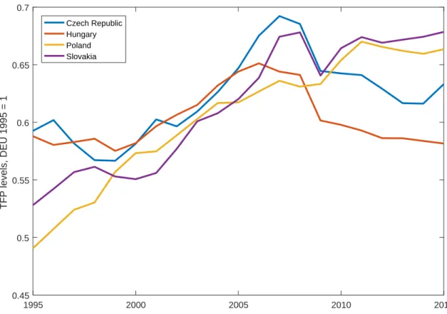
Since estimated TFP in the data is well below - but was converging to - the German level over the whole period, at least part of the convergence process was driven by productivity catch-up.

Our deterministic simulation will thus include TFP growth as a driving force. To calibrate this, we fit an AR(1) process on the panel of relative TFP paths of the Visegrad countries. We estimate the following process:

logA^j_t = (1−ρ_{tf p}) log ¯A^j+ρ_{tf p}logA^j_t−1+ν_t^{tf p},

whereA^j_t is thenormalizedTFP of countryjand timet, andA¯^jis the long run value of relative productivity. The normalization is done with average German TFP growth, i.e. the original TFP numbers are divided byg¯^t−1995, where g¯ = 1.0132 in the data. Thus our TFP series can be viewed as relative numbers compared to the steady state German path. Our GDP per capita data is normalized the same way.

Note that instead of assuming that the Visegrad countries are catching up to German TFP, we let the data tell us if this seems to be the case in the sample period. As Figure 3.1 shows, , convergence is only partial, at least in the sample period. The estimated autoregressive pa- rameters and steady state levels are given as follows:ρtf p = 0.88andA¯ = 0.637for the Czech Republic,ρ_{tf p} = 0.893andA¯= 0.60for Hungary,ρ_{tf p} = 0.889andA¯= 0.68for Poland, and ρ_{tf p} = 0.924andA¯= 0.719for Slovakia.

The other parameter values are motivated by the literature, and chosen so that we get a good fit for the convergence paths. At this point we do this informally, but in the future we are planning to employ a moment fitting exercise, at least for the key parameters. The remaining parameter values currently used are: φ = 5, ψ = 0.05,χ = 0.5, and ν = 5.³ The initial conditions

3The parameter for the debt sensitivity of the interest rate is higher than the linear estimate of Brzoza-Brzezina et al. (2016), but well below numbers found in García-Cicco, Pancrazi and Uribe (2010). It is reasonable to assume both that the degree of non-linearity in the debt - interest rate relationship is higher than in our specification, and also that the parameter might be subject to regime switches (Benczúr and Kónya, 2016). We plan to extend our model in this

1995 2000 2005 2010 2015 0.45

0.5 0.55 0.6 0.65 0.7

TFP levels, DEU 1995 = 1

Czech Republic Hungary Poland Slovakia

Figure 1: The evolution of total factor productivity in the Visegrad countries

for the simulation are as follows. The initial indebtedness relative to GDP is0.4for the Czech Republic,0.6for Hungary,0.5for Poland, and0.2for Slovakia. With the exception of Hungary, these are higher than the NFA positions in 1995. It is hard, however, to determine how different components of the NFA are viewed by financial markets when determining the appropriate risk premium for a country. Therefore, we use initial debt levels that lead to reasonable fits for the early evolution of the trade balance. Also note that in 1995, Hungary was well ahead of the other economies in foreign direct investment, which means that its NFA composition was more favorable, despite being higher in absolute level. Motivated by the Maastricht criterium, we set the steady state level of debt at0.6.⁴

Initial consumption and investment shares come directly from the data. Government spend- ing T_t is set to its sample average, which is 0.1for all countries. Total hours are normalized to1for Germany in 1995, and are appropriately transformed for the Visegrad economies using their observations. Values forθ are chosen so that the simulation matches average hours. For

direction.

4The Maastricht criterium applies to public debt, and not the the net foreign asset position. We do not make this distinction in our model, just as we do not have separate public and private debt. Our results are not particularly sensitive to the exact choice of the steady state NFA position.

the inverse Frisch elasticity of labor supply, we useϕ= 0.6. Finally, the discount factor is set to β= 0.96.

3.2 Results

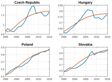
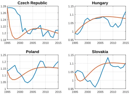
The simulation results for GDP per capita are presented on Figure 2, together with the data.

There are a couple of interesting findings. First, the model does a good job of matching the overall performance of the Visegrad countries, but there are large and lasting deviations at the country level. Our interpretation is that the countries were subject to different, persistent shocks in the sample period. In a later section we investigate this explanation, and try to recover the shocks that explain the deviations.

1995 2000 2005 2010 2015

0.9 1 1.1 1.2

Czech Republic

1995 2000 2005 2010 2015

0.6 0.65 0.7 0.75 0.8 0.85

Hungary

1995 2000 2005 2010 2015

0.5 0.6 0.7 0.8 0.9

Poland

1995 2000 2005 2010 2015

0.5 0.6 0.7 0.8 0.9 1

Slovakia

Figure 2: GDP per capita: data and simulation

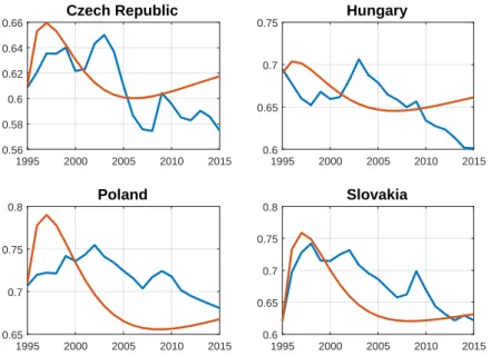
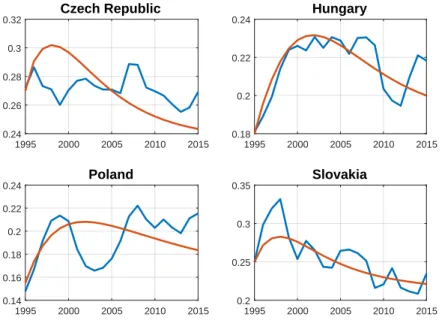
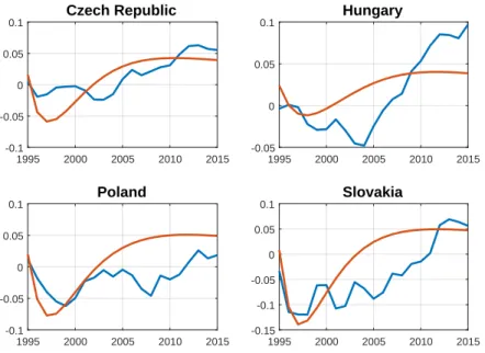
Simulation results for the three expenditure shares are depicted on Figures 3-5. The fit overall is good, but there are some persistent deviations from the predicted path. Investment is matched reasonably well, except for Poland between 2000-2006, and the model cannot quite explain the stability of the Czech investment rate. The trade balance is first over-, than under-predicted in Hungary. In Poland, consumption is higher then predicted, and consequently the trade balance is lower than predicted after 2000. These deviations are attributed - by definition - to persistent

1995 2000 2005 2010 2015 0.56

0.58 0.6 0.62 0.64 0.66

Czech Republic

1995 2000 2005 2010 2015

0.6 0.65 0.7 0.75

Hungary

1995 2000 2005 2010 2015

0.65 0.7 0.75

0.8 Poland

1995 2000 2005 2010 2015

0.6 0.65 0.7 0.75

0.8 Slovakia

Figure 3: Consumption-GDP ratio: data and simulations

1995 2000 2005 2010 2015

0.24 0.26 0.28 0.3 0.32

Czech Republic

1995 2000 2005 2010 2015

0.18 0.2 0.22 0.24

Hungary

1995 2000 2005 2010 2015

0.14 0.16 0.18 0.2 0.22 0.24

Poland

1995 2000 2005 2010 2015

0.2 0.25 0.3 0.35

Slovakia

Figure 4: Investment-GDP ratio: data and simulations

1995 2000 2005 2010 2015 -0.1

-0.05 0 0.05 0.1

Czech Republic

1995 2000 2005 2010 2015

-0.05 0 0.05 0.1

Hungary

1995 2000 2005 2010 2015

-0.1 -0.05 0 0.05

0.1 Poland

1995 2000 2005 2010 2015

-0.15 -0.1 -0.05 0 0.05

0.1 Slovakia

Figure 5: Trade balance per GDP: data and simulations

1995 2000 2005 2010 2015

1.18 1.2 1.22 1.24 1.26 1.28

Czech Republic

1995 2000 2005 2010 2015

0.95 1 1.05 1.1 1.15

Hungary

1995 2000 2005 2010 2015

1 1.05 1.1 1.15 1.2 1.25

Poland

1995 2000 2005 2010 2015

0.95 1 1.05 1.1 1.15

Slovakia

Figure 6: Aggregate hours: data and simulations

shocks to be estimated in the next section.

Finally, Figure 6 present total hours. They are well matched for Hungary, and for the Czech republic after 2000. There are fairly big temporary deviations in Slovakia and Poland, and in the Czech Republic in the first years of the sample. Again, our next exercise is to decompose these deviations into the effects of various random shocks.

4 Shock estimation

In order to estimate the stochastic shocks, we log-linearize the equilibrium conditions in (2) around the deterministic steady state. We use the five variables described in the previous sec- tion: GDP per capita, consumption, investment, and the trade balance as shares in GDP, and total hours. Since the log-linearized model is ill-equipped to explain convergence behavior when the initial conditions are far from steady state (which is the case in our economies), we subtract the fitted non-linear deterministic paths from the data, as in Figures 2-6. Note that we use log devia- tions for GDP per capita, consumption, investment and hours, but simple deviations for the trade balance, since the latter can also take on negative values. Naturally, the same transformations are applied to the model equations.

4.1 Estimation results

We do not reestimate the structural parameters. Our goal is to provide a unified framework that can account for both long-run convergence and short-run fluctuations. We thus use the same calibration as in the previous section, but estimate the four structural shocks that drive our stochastic model economy. These shocks are disturbances to the level (a_t) and growth rates (g_t) of technology, to government spending (Tt), to the interest premium (^r_t), and to labor supply.

Motivated by Garcia-Cicco, Pancrazzi and Uribe (2010), we are particularly interested in the role of the interest premium in explaining deviations from the deterministic convergence path.

The model is estimated using Bayesian techniques (An and Schorfheide, 2007). We impose flat (uniform) priors on all shock persistences on the the[0,1]interval, and assume that these parameters are the same across the four countries. We allow, however, for country-specific in-

novations. More precisely, we use the following assumptions:

a_j,t=ρ_aaj,t−1+ν_t^a+ζ_j,t^a logg_j,t=ρ_gloggj,t−1+ν_t^g+ζ_j,t^g

^r_j,t=ρr^r_j,t−1+ν_t^r+ζ_j,t^r

logT_j,t= (1−ρ_τ) log ¯T +ρ_τlogTj,t−1+ζ_j,t^τ logθt=ρhlog ¯θ+ρhlogθt−1+ζ_j,t^h

We thus allow for both a local and a regional component for the productivity and interest rate shocks, but only for local innovations for the government spending shock and the labor supply shock. We are trying to uncover the extent to which the main shocks were common across the Visegrad economies, and the extent to which the different behavior observed in the data is driven by initial conditions as opposed to different local shocks. We use flat priors for all the standard deviations of the - global or local - innovations, with a range of[0,0.2].

Table 1 contains the estimation results. The shock processes are fairly precisely estimated.⁵ The shocks are quite persistent, but clearly identified within the bounds. It is noteworthy to emphasize that although our sample period is short, and we use flat priors, the data is informative about the parameter values.

4.2 Interest rate and interest premium

In our estimation we do not use observed interest rates, rather we back them out from the evo- lution of GDP components. It is interesting to see whether these implicit interest rates “make sense”, i.e. whether their paths are in line with our prior expectations. We would like to find the following patterns: high values in the 1990s, a gradual decline before the financial crisis (espe- cially in the 2004-2008) period, and increased heterogeneity after the crisis. For the latter period, we expect interest rate increases for more heavily indebted countries (Hungary), and decreases for less indebted countries (the Czech Republic, and to a lesser extent Poland and Slovakia). It is important to note that our implicit interest rates condense price and non-price information that is relevant for intertemporal consumption and investment decisions, and thus can be quite

5Prior and posterior distributions are available from the authors upon request. Since estimated government shocks are relatively large, we experimented with a prior interval of 0-0.4. The results were unchanged, so we present the original specification in the table.

Table 1: Bayesian estimation priors and results

Prior mean Post. mean 90% conf. int. Prior Prior range AR(1) coefficients

ρ_a 0.495 0.870 0.812 0.932 Uniform 0−1

ρ_g 0.495 0.361 0.302 0.421 Uniform 0−1

ρr 0.495 0.924 0.870 0.989 Uniform 0−1

ρτ 0.495 0.828 0.703 0.971 Uniform 0−1

ρ_h 0.495 0.803 0.702 0.909 Uniform 0−1

Standard deviations Global

ν^a 0.1 0.018 0.011 0.025 Uniform 0−0.2

ν^g 0.1 0.035 0.014 0.057 Uniform 0−0.2

ν^r 0.1 0.006 0.004 0.009 Uniform 0−0.2

Czech Republic

ζ_cz^a 0.1 0.022 0.013 0.031 Uniform 0−0.2

ζcz^g 0.1 0.059 0.038 0.079 Uniform 0−0.2

ζ_cz^r 0.1 0.003 0.00 0.006 Uniform 0−0.2

ζ_cz^τ 0.1 0.090 0.065 0.114 Uniform 0−0.2

ζ_cz^h 0.1 0.053 0.021 0.087 Uniform 0−0.2

Hungary

ζ_hu^a 0.1 0.012 0.001 0.020 Uniform 0−0.2

ζ_hu^g 0.1 0.056 0.037 0.075 Uniform 0−0.2

ζ_hu^r 0.1 0.007 0.004 0.009 Uniform 0−0.2

ζ_hu^τ 0.1 0.147 0.113 0.183 Uniform 0−0.2

ζ_hu^h 0.1 0.098 0.062 0.132 Uniform 0−0.2

Poland

ζ_pl^a 0.1 0.015 0.005 0.024 Uniform 0−0.2

ζ_pl^g 0.1 0.073 0.049 0.095 Uniform 0−0.2

ζ_pl^r 0.1 0.006 0.003 0.001 Uniform 0−0.2

ζ_pl^τ 0.1 0.117 0.086 0.146 Uniform 0−0.2

ζ_pl^h 0.1 0.118 0.082 0.154 Uniform 0−0.2

Slovakia

ζ_sk^a 0.1 0.022 0.01 0.035 Uniform 0−0.2

ζ_sk^g 0.1 0.130 0.093 0.167 Uniform 0−0.2

ζ_sk^r 0.1 0.013 0.007 0.018 Uniform 0−0.2

ζ_sk^τ 0.1 0.163 0.135 0.197 Uniform 0−0.2

ζ_sk^h 0.1 0.154 0.12 0.195 Uniform 0−0.2

different from the policy rate. This is especially relevant after the financial crisis, when quanti- tative restrictions on credit became much more important, and low headline interest rates may mask high effective borrowing rates by households and small enterprises.

1995 1997 1999 2001 2003 2005 2007 2009 2011 2013 2015 Years

-4 -3 -2 -1 0 1 2 3 4

%

Implied real interest rates

Czech Republic Hungary Poland Slovakia

Figure 7: Estimated implicit interest rates

Figure 7 present the results. These are broadly in line with our expectations, with some im- portant exceptions. Before the crisis, interest rates were declining in all countries, although there is a mild reversal in the Czech Republic and Hungary after 2003. The crisis led to a significant increase in three countries. This was steepest in Hungary, which was the most heavily indebted economy, and was most exposed to financial market tightening and balance sheet adjustment.

Slovakia, as a member of the Eurozone, was hit by the subseqent Euro crisis in 2011, but the im- plcit rate came down by 2014. The Polish implicit rate remained relatively low, probably because Poland has a much bigger economy, and hence it is less exposed to external financial shocks.⁶

Given our shock specifications, we can decompose interest rate innovations into a global and

6The estimated implicit interest rates are quite high, especially compared with central bank policy rates during most of the period. This is true for the basic, representative agent real models (and many of their extensions), this has been highlighted by Mehra and Prescott (1985) as the risk-free rate puzzle. Note, on the other hand, that our implicit rate includes all price and non-price factors that influence the saving and investment decision, such as average premia on household and business lending, and/or credit rationing.

local component. The global component is dominant in the Czech Republic, while in Hungary and Slovakia the the local component is bigger. Poland is an intermediate case, where the local component was important in the middle of the sample period.

1995 2000 2005 2010 2015

Years -0.01

-0.005 0 0.005 0.01 0.015

%

Czech Republic

1995 2000 2005 2010 2015

Years -0.015

-0.01 -0.005 0 0.005 0.01 0.015

%

Hungary

1995 2000 2005 2010 2015

Years -0.01

-0.005 0 0.005 0.01 0.015 0.02

%

Poland

1995 2000 2005 2010 2015

Years -0.03

-0.02 -0.01 0 0.01 0.02

%

Slovakia

Global Domestic

Figure 8: Global and local premium shocks

The global component mostly confirms to the key developments in the region. Joining the European Union in 2004 shows up as a large decline in the effective rate. The financial crisis initially led to a small decline in the headline interest rates, but then the secondary Eurozone crisis from 2011 is likely to be behind the positive shock innovations recently.⁷ Overall, after 2005 local developments - or heterogeneous reactions to common shocks - seem to have been dominated interest rate movements in the region. This is in line with our expectations that although Visegrad countries share a similar economic structure, the financial crisis hit them differently given their external vulnerability.

7We omit the decomposition of the technology shocks for brevity. The general message is that local shocks are somewhat more important for each country, and that the global components generally follow the cyclical patterns in Europe.

4.3 Historical shocks

Our final exercise is to decompose fluctuations in GDP per capita and in the expenditure items into contributions of various shock innovations.⁸ To economize on the figures, we combine all global components into a single shock. We also merge the two technology shocks: since the transitory component is also long-lasting, we simply interpret the combined shock as a persis- tent shock to expected income. We thus have five items: “Global”, “Productivity”, “Premium”,

“Government” and “Labor” shocks. Initial conditions are also represented, which imply that ac- cording to the estimates, some variables may not have been in the steady state at the beginning of the sample period. While we removed an important reason for such findings (convergence dy- namics), it is still possible that the statistical procedure find significant deviations for the initial steady state.

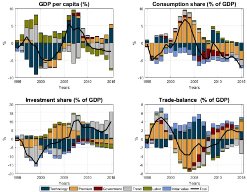
Figure 9: Shock decompositions for the Czech Republic

Figure 9 shows the Czech results. GDP per capita is mostly driven by productivity, and to a lesser extent labor market, shocks. Productivity is the most siginificant driver of investment, al- though (global) premium shocks helped in the first half of the 2000s. Consumption and the trade

8We omit the shock decomposition of total hours, the result are available form the authors upon request.

balance are driven largely by global premium shocks. Interestingly, as we saw above, local pre- mium shocks are almost irrelevant in the Czech Republic, except around the financial crisis. This result confirms that for a less indebted economy premium shocks are not particularly important.

Figure 10: Shock decompositions for Hungary

Hungarian results are depicted on Figure 10. They show a quite different pattern: as opposed to the Czech Republic, (local and global) premium shocks are very important for the evolution of consumption, the trade balance, and investment. The Hungarian economy was fueled by cheap credit before the crisis, and it had to go through a significant balance sheet adjustment post-crisis.

Interestingly, while premium shocks are largely responsible for the composition of GDP, output itself was driven more by productivity, although labor shocks and premium shocks were impor- tant during the crisis years as well. The shock decomposition of investment between 2000-2009 tells an interesting story, which is in line with our prior about the Hungarian economy. In this period, increasingly negative growth prospects were countered by a favorable external finan- cial environment. We can also see that between 2006-2008, when the global financial conditions started to become more restrictive, local premium shocks were significantly negative (Figure 8).

This was the period when Hungarian firms and households increasingly turned to foreign inter-

est loans. Finally, investment increases in the last three years are also attributed to productivity shocks, but detailed information reveals that this is mostly government investment based on EU funding. We plan to investigate the role of the government further in the future.

Figure 11: Shock decompositions for Poland

Similarly to the Czech Republic, labor and productivity shocks are driving GDP per capita in Poland (Figure 11), but in exactly the opposite direction. Productivity shocks operated mostly through investment, especially during its big collapse after 2000. In the last decade, favorable premium shocks led to increases in both consumption and investment, at the cost of a declining trade balance. The impact of global shocks is small in Poland, probably because it is by far the largest economy in the region.

Finally, Figure 12 presents the Slovakian results. All shocks contributed to the evolution of GDP per capita, while the premium shock is important for the GDP components. As in Poland, investment seems to have been aided recently by favorable premium shocks, and hindered by productivity shocks.

To sum up, premium shocks play a significant role in most countries, especially for the ex- penditure components. Hungary is the most clear-cut case: since it was by far the most heavily

Figure 12: Shock decompositions for Slovakia

indebted before the crisis, external premium shocks had the largest impact on its economy (see also Benczúr and Kónya, 2016). Productivity shocks and labor market shocks drive GDP per capita, but the cross-country pattern is quite heterogeneous. Global shocks overall had a moder- ate impact in the Visegrad countries, with the Czech Republic being the most affected in relative terms. Looking at the scale of the fluctuations, this just means that local shocks were the smallest in the Czech Republic, hence the decomposition gives relatively more weight to global ones.

5 Conclusion

In this paper we used a version of the neoclassical growth model to understand the stochastic convergence process of the Visegrad economies in a unified framework. Our findings indicate that the neoclassical model, augmented with financial frictions, is a good starting point to under- stand the growth process of the Visegrad economies. Initial conditions and long-run productivity convergence do a good job in explaining the growth paths of the four countries. Significant de- viations can be seen, however, which indicate that external shocks were hitting the countries as

well. In the second part of the paper we estimated the relative importance of technology, interest premium, government and labor supply shocks. We also allowed for a global component for the first two.

In our empirical exercise we find mixed results. Productivity shocks are important in some cases, especially for the overall level of GDP per capita. Interest premium shocks are impor- tant drivers of consumption, investment and the trade balance, especially in the most heavily indebted country, Hungary. TFP shocks are lasting, and our estimation suggests that technology or income expectation are very persistent. Overall, our results suggest that individual country performances were driven mostly by local conditions. Many open questions remain for further research, including the role of EU funding. The model developed and estimate in this paper seems to be a good starting point to understand the growth performance of the Visegrad economies.

References

Aguiar, M. és Gopinath, G. (2007). “Emerging Market Business Cycles: The Cycle Is the Trend.”

Journal of Political Economy,115: 69–102.

An, S. és Schorfheide, F. (2007). “Bayesian Analysis of DSGE Models.”Econometric Reviews,26: 113–172.

Benczúr, P. and I. Kónya (2016). “Interest premium, sudden stop, and adjustment in a small open economy.”Eastern European Economics,54: 271-295.

Brzoza-Brzezina, M. and J. Kotlowski (2016). “The nonlinear nature of country risk.” National Bank of Poland, Mimeo.

Christiano, L., M. Eichenbaum and C. Evans (2005). “Nominal Rigidities and the Dynamic Effects of a Shock to Monetary Policy.”Journal of Political Economy,113: 1-45.

García-Cicco, J., Pancrazi, R. és Uribe, M. (2010). “Real Business Cycles in Emerging Countries?”

American Economic Review,100: 2510–2531.

Gollin, D (2002). “Getting Income Shares Right.”Journal of Political Economy,110: 458-474.

Guerron-Quintana, P. (2013). “Common and idiosyncratic disturbances in developed small open economies.”Journal of International Economics,90: 33-49.

Kónya, I. (2013). “Development Accounting with Wedges: the Experience of Six European Coun- tries.”The B.E. Journal of Macroeconomics(Contributions),13:245-286

Mehra, R. and E. Prescott (1985). “The equity premium: A puzzle.”Journal of Monetary Eco- nomics,2: 145-161.

Minetti, R. és T. Peng (2013). “Lending constraints, real estate prices and business cycles in emerging economies.”Journal of Economic Dynamics & Control,37: 2397–2416.

Naoussi, C. és F. Tripier (2013). “„Trend shocks and economic development.”Journal of Develop- ment Economics,103: 29-42.

Schmitt-Grohé, S. és Uribe, M. (2003). “„Closing small open economy models.”Journal of Inter- national Economics,61: 163–185.

Tastan, H. (2013). “Real business cycles in emerging economies: Turkish case.”Economic Mod- elling,34: 106-113.

Valentinyi, Á. and B. Herrendorf (2008). “Measuring Factor Income Shares at the Sector Level.”

Review of Economic Dynamics,11: 820-835.

Zhao, Y. (2013). “Borrowing constraints and the trade balance–output comovement.”Economic Modelling,32: 34-41.A