Be; ¯Jk The cost function of the ith player; Average cost of players in kthNash equilibrium. SDk,j A joint decision vector of all players in the kth subgame of the jth game.
Background
Traffic Light Control
According to the adaptability and intelligence level of the system, STLCS can be classified into five levels (Gartner et al., 1995). Similar to the second-level STLCS, the third-level STLCS is able to adjust the parameters based on the situation of the time-varying traffic flow (Lee et al., 2019).
Traffic Lane-changing Control
In general, in rule-based models, the lane changer changes lanes only when the target lane has an available gap, reducing efficiency when changing lanes in heavy traffic. Integrating artificial intelligence into the lane change system is a promising direction in recent research.
Research Methodology
Traffic Light Models
Usually, the traffic signal control problem situation is formulated as an MDP (Xu et al., 2016; Zhang and Prieur, 2017), where the states only depend on the agents' actions. Previous work introduces a simple case of isolated traffic signal control involving the application of RL (Abdulhai et al., 2003) and applies RL to prove the effectiveness and efficiency of traffic control (Bazzan, 2009).
Traffic Lane-changing Models
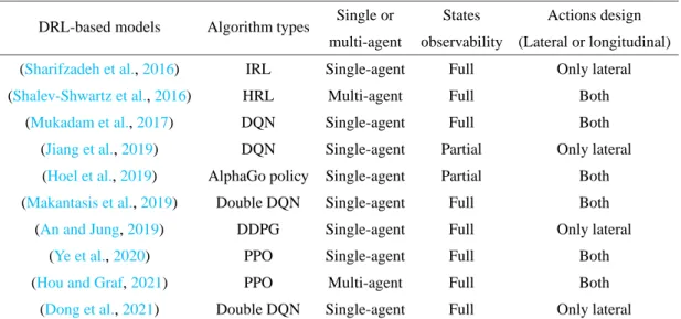
The recent DRL-based lane-changing models summarized in Table 1.1 overcome the problem of game theory-based lane-changing models (i.e. long computation time with a large number of players). Although (Hou and Graf, 2021) model the lane-changing system as a multi-agent system, it is performed in a decentralized manner.
Thesis Outline
Games and Definitions
Each entry of the matrix ai j is an outcome (ie cost) corresponding to the joint decisions made by the players. In most cases, the real problem of a complex environment can be constructed as a non-cooperative non-zero-sum N-person game.
Nash Equilibrium
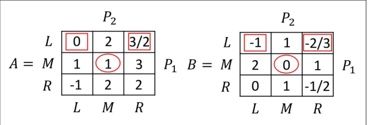
Stackelberg Equilibrium
According to these pairs of decisions, {L} is the most rational choice for the leader P1 because of the lowest cost. The same steps are applied to find the Stackelberg equilibrium solution in the case where P2 is leader and {L,R} is the solution.
Framework of Reinforcement Learning
- Basic Definitions
- Markov Decision Process
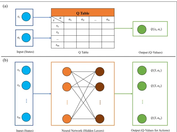
- Q-learning
- Deep Q-learning
A Markov process is also called a Markov chain, that is, a memoryless random process with the Markov property (i.e. the future is independent of the past given the present). In (3.5) the minus part−gwizj(k)OwizjTs follows the speed of outgoing traffic flow, even though there are still some vehicles that have not been removed on the road.

Game Theoretical Strategies
Global Optimal Strategy
Nash Equilibrium Strategy
Stackelberg Equilibrium Strategy
Experiments
Parameters
Results
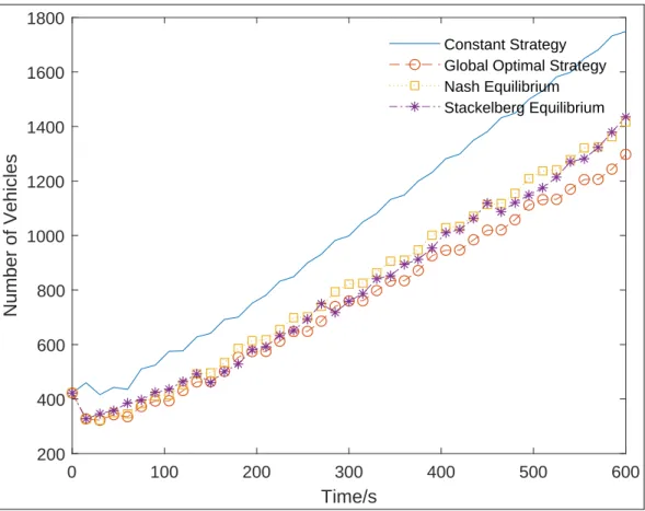
In Figure 3.2 with the constant control strategy, the number of vehicles in queues increases to 467 at the end of the first epoch, then gradually decreases in the second epoch, but rises sharply in the last two segments. It is clear that the curve of the first two strategies shows a similar tendency, i.e. the number of passing vehicles increases dramatically in the first time slice and bottoms out at 82 and 157 respectively, after which both increase. Finally, the number of vehicles in the queue is smallest for the global optimal strategy, then larger and similar for both Nash equilibrium and Stackelberg equilibrium strategies.

Summary
Conclusion
A similar process takes place for the Stackelberg equilibrium in the beginning, but remains stable around 130, only with a small fluctuation from the second time segment to the last segment. At the end of the cycle time, the total number of vehicles in rows of quadruple segments with the constant steering strategy, global optimal strategy, Nash equilibrium and Stackelberg equilibrium, respectively, is 385 and the total number of passing vehicles is 640. length increases as time passes, but at a different speed for these four strategies in Fig.3.4 due to the incoming flow.
Contribution
Traffic light controls are controlled automatically instead of adjusting traffic light schedules. Subsequently, the performance of the proposed algorithm and the strategies in chapter 3 are compared. In the MARL system, the state space is defined as S

Proposed Method Framework
Also, ¯Jk= 1n∑ni=1Jw∗,ki is the average cost of the players in the kth Nash equilibrium,ω1andω2are the weighting factors. Finally, we can know the unique Nash equilibrium of the combination of decisions is (dw∗,k1∗,dw∗,k2∗,dw∗,k3∗,dw∗,k4∗) respectively for the players. The number of actions of agent ai is defined as |ai|, so the size of joint action space is |A|=.
Experiments
Parameters
Results
Each curve represents the Q-values of an agent taking joint actions based on a Nash equilibrium. All curves tend to converge as the iterations increase, and eventually the optimal joint actions corresponding to the Nash equilibrium will be selected. Meanwhile, compared to Figure 4.2, the Q-values of SNAQ converge earlier and more stably with the same iterations.

Summary
Conclusion
Table 4.3 compares the performance, such as average queues and average throughput (i.e. passing vehicles in a certain period) among all traffic light control strategies. Compared with strategies in Chapter 3, shown in Table 4.3, SSBQ shows almost the best performance as the game theory-based strategies in Chapter 3 in traffic light control. However, SSBQ, which is the RL method, spends much less time on computation in the execution process due to the learning ability compared to the game theory-based strategies, which is the main advantage of the learning system.
Contribution
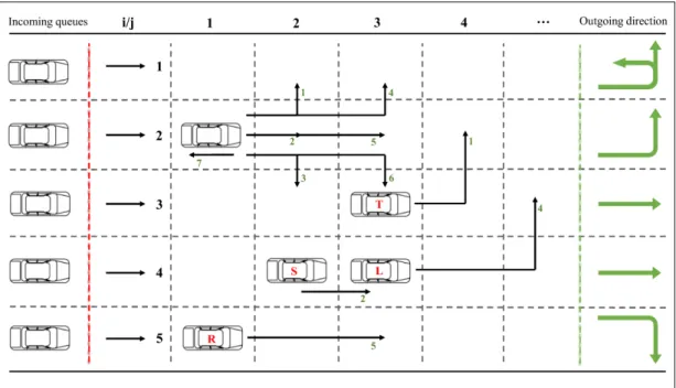
This lane change system can be divided into three sectors, i.e. the inbound sector after the red line, the outbound sector before the green line and the lane change sector in between. In the middle, i.e., the lane change sector, which can be constructed as a Cel matrix from the point of view of mathematics. Elements such as T: U turn, L: left turn, R: right turn, S: straight are the target lane values, which can be converted to a digital number (ie, the target lane index).
Decision-making Strategies
Gap Acceptance Strategy
Initialization: initialize the current coordinate Celi,j of each individual vehicle, the current lane index i∈ΩN={1,2,.
Classic Nash Equilibrium Strategy
The absolute difference between the target Tagi band and the current i band indicates how much the vehicle wants the MLC to reduce the distance. The utility value increases as the vehicle approaches the target lane and the vehicle stays in the target lane if the difference is zero (ie, maximum). In the second part, ω2≪ω1 and ∑n−j jCeli,ji is the queue in front of vehicle Celi,j.
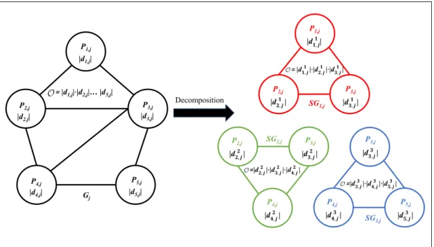
Decomposition Algorithm
The combination of these decisions also maximizes the utility value of the corresponding players in the game Gj, which is proved and deduced from Theorem 5.1. Then, the optimal decisions of the remaining players in the game Gj will be chosen in a certain direction based on Epc∗,1, which means that the neighboring player will update the decision with the collision constraints prorogued by the previous subgames. The update direction of E–‰Ú The update direction of E–‰Û The update direction of E–‰Ü The subgames of E–‰Ú The subgames of E–‰Û The subgames of E–‰Ü. 5.5: Schematic of the PCE update process.
Simulation
- Experimental Setup
- Examples of Lane-changes Maneuvers
- Comparison in a Single Test
- Comparison in Multiple Tests
Throughput indicates how much traffic flow passes through the lane change sector in a given unit period, which is directly related to passing vehicles and is expressed as PV/T (i.e. number of passing vehicles per iteration). Therefore, more vehicles in the lane change sector would reduce their speed, resulting in the accumulation of inbound queues in the inbound queue sector. The number of lane-changing vehicles and the average computation time per iteration can be obtained at the end of the simulation.
Discussion
This results in a slightly better performance in S3 than S2 in lane changing efficiency after a long period. As it grows, the number of game players increases dramatically with more vehicles in the lane changing sector. According to Algorithm 5.1, the complexity of S1 is also determined by the number of vehicles in the lane change sector.
Summary
Conclusion
First, some assumptions are still ideal in this proposed model, such as the discrete space of lanes, the discrete speed of vehicles, and the smooth operational maneuvers. In addition, if the players do not know the identified connections with neighboring players, it is limited to parsing a large game into several smaller games. Finally, it is not very suitable for dissecting a three-dimensional game, since the interactions between players are quite complicated, for example, controlling an unmanned aerial vehicle system.
Contribution
A normal lane changing system contains five lanes, which can be divided into cells shown in Fig.6.1. Fig. 6.1 shows examples of performing an action by the vehicle, e.g. the vehicle with an element L in position Cel3,2 intends to change to target lane 1 or 2 with action turn left. It is assumed that the vehicles can pass smoothly across each other even with parts of the lane overlapping (e.g. the vehicle at position Cel4,2 can turn right and the vehicle at position Cel5,2 can turn left at the same time, shown in Fig. 6.1) .
Proposed Method Framework
As shown in Fig.6.2(b), the set j+1 in front of the request set is a response set. Get the joint actions of the group on request Ajand overlay action Cj; Construct the request message Aj+Cj;. Furthermore, a communication vector Cj is superimposed based on the joint actions of the front group.

Simulation
Experimental Setup
A variety of conditions (indicators) are defined to evaluate the performance of the path-changing approaches. The lane change maneuvers must be completed before moving through the lane change area. The agent will accelerate or decelerate to create an available gap to satisfy the lane-changing demand of the adjacent agent.

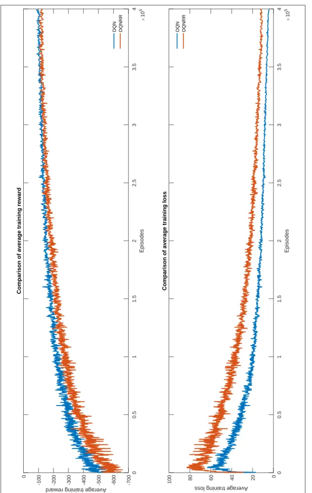
Performance of Training Process
The optimal joint actions for the same group can be selected by finding the fully consistent or partially consistent equilibrium. Thus, during the execution process, each group produces joint actions for the agents in the same group by using the trained request Q network, which is also part of the proposed method. Due to the additional reward from the request confirmation, the loss value of DQNRR is a litter higher than the loss value of DQN during the same training episode.
Evaluation of Control Methods
RMSE (i.e. root mean square error) measures the difference between predicted values and observed values (Hyndman and Koehler, 2006) and residual histograms (i.e. the area of each bar is the relative number of observations and the sum of bar areas equals 1) shows whether the residuals are normally distributed. However, the value of DQN is smaller than the other two, and the residuals are distributed worse than the others. In this regression model, R-squared = 0 represents the y-axis value (i.e. computation time) has no correlation with x-axis value (i.e. the expected traffic density).
Discussion
Indeed, the control mechanism of these methods is the critical element of this lane change system and determines the value of Lr. The lane change rate decreases exponentially as the expected traffic densityρ increases, which corresponds to the property in Figure 6.5. Unlike the other three methods that hold Lr with different ρ (i.e., ρ is below the control limit of these methods), the RULE method has the worst ability to control traffic flow in stalled traffic (for example, the value decreases exponentially when ρ exceeds 0.54, shown in Fig. 6.7).
Summary
Conclusion
Contribution
Specifically, the request group trains agents by considering only the states of the group, while the response group also evaluates the superimposed actions (i.e., the request message) of the request group in addition to the states of the group. The last thesis in this paper is the application of MARL in the traffic lane changing system. Nevertheless, the limitations of the trajectory-changing model are the same as in the previous thesis mentioned above.
Future Work
A game theory-based approach to modeling mandatory lane-changing behavior in a connected environment. A game theory-based approach to modeling autonomous vehicle behavior in congested, urban lane-changing scenarios. Traffic lane-changing modeling and planning with game-theoretic strategy, in: 2021 25th International Conference on Methods and Models in Automation and Robotics (MMAR), IEEE.

Example of Nash equilibrium in a bimatrix game
Example of Stackel equilibrium in a bimatrix game
A schematic of agent-environment interaction
A example of Markov chain
The structure of Q-learning and deep Q-learning
General structure of the intersection
Vehicles in queues (total) with four strategies in 1 cycle
Passed vehicles (total) with four strategies in 1 cycle
Vehicles in queues (total) with four strategies in 10 cycles
Passed vehicles (total) with four strategies in 10 cycles
Comparison of waiting vehicles "Queues" in 20 time slices
The schematic of the lane-changing system
Collision cases in the lane-changing system. (a) Position collision of
The graphic process of decomposing games
The schematic of decomposing games in the lane-changing system
The schematic of the updating process of PCE
Existing lane-changing models based on deep reinforcement learning
Decimal decisions and calculation time of four strategies in 1 cycle
State space
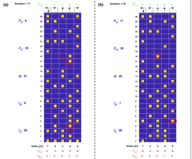
States comparison in two MARL Algorithms
Comparison of all traffic light control strategies in 5 cycle
Actions of vehicles
Comparison of states between the strategies in multiple tests
Basic actions of vehicles
Extended actions of vehicles
List of hyperparameters of the training process in both learning algorithms105