https://doi.org/10.1007/s12190-019-01250-5 O R I G I N A L R E S E A R C H
Global dynamics of a mathematical model for a honeybee colony infested by virus-carrying Varroa mites
Attila Dénes1 ·Mahmoud A. Ibrahim1,2
Received: 27 November 2018
© The Author(s) 2019
Abstract
We establish a new four-dimensional system of differential equations for a honeybee colony to simultaneously model the spread ofVarroamites among the bees and the spread of a virus transmitted by the mites. The bee population is divided to forager and hive bees, while the latter are further divided into three compartments: suscepti- bles, those infested by non-infectious vectors and those infested by infectious vectors.
The system has four potential equilibria. We identify three reproduction numbers that determine the global asymptotic stability of the four possible equilibria. By using Dulac’s criterion, Poincaré–Bendixson and persistence theory, we show that the solu- tions always converge to one of the equilibria, depending on those three reproduction numbers. Hence we completely describe the global dynamics of the system.
Keywords Epidemic model·Honeybees·Varroainfestation·Global stability· Persistence
Mathematics Subject Classification 34D23·92D30
1 Introduction
Honeybee is a member of the genusApiswhich produces and stores honey and con- structs perennial, colonial nests from wax. The best known species of the genus is the Western honey bee (Apis mellifera, also called European or common honey bee) which was domesticated for honey production and crop pollination or at least exploited for honey and beeswax [1] at least since the time of the building of the Egyptian pyramids.
A. melliferais the only species that has been moved extensively beyond its native ter-
B
Mahmoud A. Ibrahim mibrahim@math.u-szeged.hu1 Bolyai Institute, University of Szeged, Aradi vértanúk tere 1, Szeged 6720, Hungary
2 Department of Mathematics, Faculty of Science, Mansoura University, Mansoura 35516, Egypt
ritory. Aside from their ecological importance [2], honey bee populations have a large economical impact on agriculture in the whole world [3–5].
Colony collapse disorder (CCD) is the phenomenon of the majority of worker bees in a colony disappearing and leaving behind a queen, plenty of food and some nurse bees to care for the remaining immature bees. The phenomenon was renamed colony collapse disorder in 2006 when abnormally high die-offs (30–70% of hives) of common honeybee colonies have occurred in North America and at first no explanation could be given [6]. Several European countries have experienced the same phenomenon since 1998, and in the past few years countries in Africa and Asia also became affected by it. The reason seems to be a combination of factors, possibly including neonicotinoid pesticides or Israeli acute paralysis virus [7]. The collapse of honeybee colonies has become widespread in several regions of the world, and has been the subject of much discussion and research in recent years [8–10].
Varroamite is an external parasitic mite that attacks the honey beesApis ceranaand Apis mellifera. It attaches to the body of the bee and weakens the bee by sucking fat bodies [11]. A significant mite infestation will lead to the death of a honey bee colony, usually in the late autumn through early spring. TheVarroamite is the parasite with the most pronounced economic impact on the beekeeping industry. Also, it is considered to be one of multiple stress factors [12] contributing to the higher levels of bee losses around the world.Varroamites are carriers for many viruses that are damaging to bees, including Kashmir bee virus, sac-brood virus, acute bee paralysis virus, Israeli acuteparalysis virus, and deformed wing virus [13].
Several methods of treatment are currently applied to control these mites, which can be divided into chemical and mechanical controls. Usual chemical controls include
“hard” synthetic chemicals such as amitraz, fluvalinate and coumaphos, while “soft”
chemical controls (organic acids, essential oils) include thymol, sucrose octanoate esters oxalic acid and formic acid. Mechanical controls are usually based on disruption of some aspect of the mites’ life cycle and they are generally intended not to eliminate all mites, but to keep the infestation at a tolerable level. Examples of mechanical controls include sacrifice of drone brood asVarroamites most commonly attach to the drone brood, powdered sugar dusting which encourages cleaning behaviour and dislodges part of the mites, screened bottom boards which allows dislodged mites to fall through the bottom and away from the colony, brood interruption, application of heat to isolated brood combs or whole colonies and downsizing of the brood cell size.
Another possibility in fighting the infestations is breeding more resistant colonies:
several families of bees are able to coexist withVarroamites (e.g. Africanized bees and Russian honey bees show a higher natural resistance against mites) [13–15].
A number of mathematical models have been established to modelVarroainfesta- tion and associated virus infections. Sumpter et al. [16] studied the disease in honey bee colonies and modeled the effects ofVarroamites on the brood and on the adult worker bees. The focus of the model was on the relationship between the mite popu- lation within a hive and its role in virus transmission within the hive. A study by Ratti et al. [17] examined the transmission of viruses viaVarroamites with the mites as vectors for transmission. In Ratti et al. [17], the population of honeybees was divided into honeybees that are virus free and that are infected with the virus, while the same
population compartments of honeybees with adding mortality caused by mites in Ratti et al. [18].
The model presented in Kang et al. [19] follows Sumpter et al. [16] and Ratti et al. [18] with the same compartments for honeybees, but it also takes into account the fact that virus transmission occurs at different biological stages ofVarroamites and honeybees. The models of Ratti et al. [18] and Kang et al. [19] are extended in Ratti et al. [20] by introducing uninfected forager bees as a new honeybees compartment, also by adding different types of mortality.
The purpose of this work is to establish and analyse a novel mathematical model for the dynamics of a honeybee colony affected byVarroamites by providing a new approach in comparison with earlier works: instead of considering separate compart- ments for the mites, we divide the honeybees into compartments depending on their infestation and infection status, based on earlier models for ectoparasite-borne dis- eases [21–24]. In the present paper we set up the simplest model that is complex enough to capture the fundamental features of the parallel transmission of the mite infestation and the infection. The model is based on the ectoparasite model given in [22], however, in the present model we consider different birth and death rates and additional disease-induced mortality for infected bees. Most importantly, we extend the model with a new compartment by differentiating susceptible hive bees and forager bees. Hence, our model consists of four nonlinear ODEs dividing the population of hive bees into susceptible (uninfected and uninfested) hive bees, hive bees infested by non-infectious vectors and hive bees infested by infectious vectors (infected hive bees) with mortality caused by mites. The fourth compartment stands for forager bees.
We identify key variables that determine the collapse or survival of the bee colony, namely the severity of the disease and the rate of transmission, and examine different scenarios using different combinations of these variables.
The structure of the paper is the following. In Sect.2, we establish our compart- mental model describing the spread of the infestation and the disease. In Sect.3, we study the three-dimensional subsystem and determine the reproduction numbers and prove the existence of the positive equilibria. In Sect.s4and5, we investigate the local stability of equilibria and prove the persistence of the compartments, while, using the results of Sects.4and5, we study the global stability of equilibria. In the last section, we use the results of the previous sections to study the two-dimensional subsystem of susceptible.
2 Mathematical model
Our mathematical model is based on the presence of a mite species which is a vector for a disease as well and transmitted to a susceptible host only upon adequate contact with an infested host. The honeybee population is divided into four compartments depending on the presence of the vectors and the disease transmitted by them as follows.
(i) Susceptibles: those who can be infested by the vector. Following [20,25] the healthy bee population is divided into hive bees and foragers. We denote by Hs
the compartment of susceptible hive bees andFsthe compartment of susceptible forager bees.
(ii) Hmdenotes hive bees infested by non-infectious vectors.
(iii) Hi denotes hive bees infested by infectious vectors, and thus infected with the disease.
In our model we assume that the following assumptions hold.
1. Hive bees (fromHm) infested by non-infectious vectors can transmit the disease to susceptibles (hive and forager bees), hive bees infested by infectious vectors (fromHi) can transmit the disease to susceptibles (hive and forager bees).
2. We assume that once infected or infested, forager bees are forced to stop their foraging duties because of the infestation or infection and become hive bees.
3. A hive bee infested by infectious vectors can transmit the infection to a hive bee infested by non-infectious vectors, i.e. a member of compartmentHm can move to compartmentHi upon adequate contact with an individual from compartment Hi.
4. We suppose that, upon adequate contact with a susceptible bee, an individual fromHm can transmit the (non-infectious) mites carried by it at the same rate to susceptibles (Hs andFs), and we denote the transmission rate for non-infectious vectorsHmto susceptibles byβ1.
5. We assume that, upon adequate contact with a susceptible bee or a bee with non- infectious parasites, an individual from Hi can transmit the mites carrying the virus at the same rate to susceptibles (Hs andFs) and to those who are already infested by non-infectious vectorsHm. We denote this transmission rate byβ2. 6. We assume that the disinfestation rates from theHmandHi compartments to the
susceptible compartmentHsare the same and denoted byα.
7. We denote by A(Hs,Fs)the natural birth rate of healthy hive beesHs and byd the death rate for the compartmentsHs,FsandHm.
8. We assume that only infected hive bees die due to the mites transmitting viral infection. So, we assume that the death rate of infected hive beesHi is equal to d+δwhereδis the death rate caused by mites.
9. In accordance with [26], we assume that the proportion of recruitment of suscep- tible hive beesHsto become forager bees and the rate of healthy forager beesFs
that are reverting to hive duties following social inhibition has the same propor- tionR(Hs,Fs). We formulate this process of recruitment and social inhibition as a Holling-type II functional response, see [20,25,27].
Using the above assumptions, our model takes the form:
Hs(t)= A(Hs,Fs)−β1Hs(t)Hm(t)−β2Hs(t)Hi(t)+αHm(t)+αHi(t)
−d Hs(t)−R(Hs,Fs)Hs(t)+R(Hs,Fs)Fs(t),
Fs(t)=R(Hs,Fs)Hs(t)−β1Fs(t)Hm(t)−β2Fs(t)Hi(t)−d Fs(t)
−R(Hs,Fs)Fs(t),
Hm(t)=β1Hs(t)Hm(t)+β1Fs(t)Hm(t)−β2Hm(t)Hi(t)−αHm(t)
−d Hm(t),
Hi(t)=β2Hs(t)Hi(t)+β2Fs(t)Hi(t)+β2Hm(t)Hi(t)−αHi(t)
−d Hi(t)−δHi(t), (1) where the term R(Hs,Fs)in the first two equations represents the effect of social inhibition on the recruitment rate and is formulated as
R(Hs,Fs)=σ1−σ2
Fs
Hs+Fs
(2) where the parameterσ1is the maximum rate at which hive bees are recruited as foragers when there are no foragers present in the colony. The termσ2 Fs
Hs+Fs represents social inhibition, that is, the process whereby a surplus of foragers causes the foragers to revert to being hive bees. We assume that social inhibition is directly proportional to the forager population present in the colony.
In the present paper, following [16] and for technical reasons, we will consider a constant birth rate and study the special case
Hs(t)=A−β1Hs(t)Hm(t)−β2Hs(t)Hi(t)+αHm(t)+αHi(t)
−d Hs(t)−R(Hs,Fs)Hs(t)+R(Hs,Fs)Fs(t),
Fs(t)=R(Hs,Fs)Hs(t)−β1Fs(t)Hm(t)−β2Fs(t)Hi(t)−d Fs(t)
−R(Hs,Fs)Fs(t),
Hm(t)=β1Hs(t)Hm(t)+β1Fs(t)Hm(t)−β2Hm(t)Hi(t)−αHm(t)
−d Hm(t),
Hi(t)=β2Hs(t)Hi(t)+β2Fs(t)Hi(t)+β2Hm(t)Hi(t)−αHi(t)
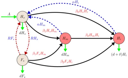
−d Hi(t)−δHi(t). (3) The transmission chart of the model is depicted in Fig.1.
Let us introduce the notation S(t) = Hs(t)+Fs(t). With this notation, we can transcribe system (3) to the three-dimensional system
S(t)= A−β1S(t)Hm(t)−β2S(t)Hi(t)+αHm(t)+αHi(t)−d S(t), Hm(t)=β1S(t)Hm(t)−β2Hm(t)Hi(t)−αHm(t)−d Hm(t),
Hi(t)=β2S(t)Hi(t)+β2Hm(t)Hi(t)−αHi(t)−d Hi(t)−δHi(t).
(4)
Let us note that this system has a similar structure as the model given by Dénes and Röst in [21,22] and the rodent subsystem given by Dénes and Röst in [23], however, in the present case, in contrary to those papers, birth and death rates are different and there is additional mortality for infected hive bees. Because of these differences in the models and to make the present paper self-contained, we give all the proofs of the results on the dynamics of model (3). We also note that the methods applied in the analysis are also different: in the earlier papers, Lyapunov functions were used in the
Hs
dHs
Fs
dFs
Hm
dHm
Hi
(d+δ)Hi
αHm
β1HsHm
RFs RHs
αHi
β1FsHm
β2FsHi
β2HmHi
A β2HsHi
Fig. 1 Transmission diagram of the dynamics of the honey bee colony combined with the dynamics of a non-infectious and infectious disease. Brown nodes are susceptible bees and red nodes are infested by non-infectious (Hm) and by infectious (Hi). Black solid arrows show the progression of infection. Blue dashed arrows show disinfestation. Red dash-dotted lines show movement between the susceptible hive bee and susceptible forager bee compartments. Green solid arrows show natural birth death. (Color figure online)
proofs of global stability, however, in the present paper we apply Bendixson–Dulac criterion instead.
3 Equilibria, reproduction numbers
To determine the equilibria of the full system (3), we start by calculating those of the subsystem (4). These are easily obtained by solving the algebraic system of equations
0= A−β1S∗Hm∗−β2S∗Hi∗+αHm∗+αHi∗−d S∗, 0=β1S∗Hm∗−β2Hm∗Hi∗−αHm∗−d Hm∗,
0=β2S∗Hi∗+β2Hm∗Hi∗−αHi∗−d Hi∗−δHi∗.
We can determine four possible equilibria of system (4), one of which is disease- and infestation-free, one is disease-free with infestation, one is endemic where all vectors are infectious, and one is endemic where both infectious and non-infectious vectors are present:
Es = A
d,0,0 , Em=
d+α
β1 ,Ad −dβ+α1 ,0 ,
Ei =
d+α+δ
β2 ,0,−d(dβ+α+δ)+2(d+δ)Aβ2 , Emi =
αδ+aβ2
β1(d+δ),(d+δ)(d+α+δ)ββ1β2(d1+δ)−β2(αδ+aβ2),−d(dβ+α+δ)+2(d+δ)Aβ2 .
(5)
Due to the biological interpretation of the model, we are only interested in non- negative equilibria. In the sequel, we say that a given equilibrium exists, if each of its three coordinates is non-negative.
We can determine four reproduction numbers by introducing a single infested (infectious or non-infectious) individual into a population in which neither infected nor non-infected parasites are present (Es), or into a population where only non- infected parasites are present (Em), or into a population where only infected parasites are present (Ei), and calculating the expected number of generated secondary cases.
If we introduce an individual infested by non-infectious mites into the infestation- and disease-free equilibriumEs, we obtain the reproduction number
R1= Aβ1
d(d+α),
by introducing an individual infested by infested mites into the same equilibrium we obtain the reproduction number
R2= Aβ2
d(d+α+δ).
Calculating the expected number of secondary infections caused by the introduction of an individual infested by infectious mites into a population in the equilibriumEm, we obtain the same reproduction numberR2, as the transmission rate fromHiindividuals is the same for theSandHmcompartment.
Finally, let us introduce an individual infested by non-infectious mites into a pop- ulation in the equilibriumEi. In this case, the expected sojourn time of an individual infected with the first strain in the Hm compartment is(β2Hi∗+α+d)−1, and the number of new infections generated by this individual is β1S∗, where S∗ and Hi∗ stand for the first, resp. Taking the product of these two expressions and substituting the values ofS∗andHi∗at the equilibriumEi, we obtain the reproduction number
R3= (d+δ)(d+α+δ)β1
β2(αδ+Aβ2) .
In the next proposition we show how the reproduction numbers determine the existence of the four equilibria.
Proposition 3.1 The equilibrium Es always exists. The equilibrium Em exists if and only if R1>1. The equilibrium Ei exists if and only if R2>1. The equilibrium Emi
exists if and only if R2>1and R3>1.
Proof The first coordinate of Em is less than dA if and only ifR1 >1. If this holds, also the second coordinate of this equilibrium is between 0 and dA. Similarly, we have that Ei exists if and only ifR2 >1, also the second coordinate of this equilibrium is between 0 and dA+δ. In the case of the equilibriumEmi, the third coordinate being between 0 and d+δA is equivalent to R2 >1. If R2 >1, then the second coordinate being positive is equivalent toR3>1. Thus for the existence ofEmi, it is necessary
that R2>1 andR3>1. To see the sufficiency, notice that Ad R1
2R3 = (αδ+d+δ)βAβ12, which is the first coordinate, thus ifR2>1 andR3>1, then the first and second coordinates ofEmi are between 0 and dAand the third between 0 andd+δA .
4 Local stability
Proposition 4.1 The stability of equilibria is determined by the reproduction numbers as follows.
(i) Esis locally asymptotically stable if R1<1and R2<1, and unstable if R1>1 and R2>1.
(ii) Emis locally asymptotically stable if R1>1and R2<1, and unstable if R1<1 and R2>1.
(iii) Eiis locally asymptotically stable if R2>1and R3<1, and unstable if R3>1.
(iv) Emi is locally asymptotically stable if R2 >1and R3>1(i.e. always when it exists).
Proof (i) The eigenvalues of the Jacobian of the linearized equation around the equilibrium Es areλS1 = −b, λS2 = −d −α+ Adβ1 =(d +α)(R1−1)and λS3 = Aβ2−d(dd+α+δ) =(d+α+δ)(R2−1). All of the eigenvalues are negative if R1 < 1 and R2 < 1, while at least one of them is positive if R1 > 1 and
R2>1.
(ii) If we linearize around the equilibriumEm, we find the eigenvaluesλHm1 =λS1, λHm2 = −λS2 andλHm3 =λS3, thus we can argue similarly as in case (i).
(iii) Linearization around the equilibriumEi yields the three eigenvalues λHi1 = (d+α+δ)β1
β2 −αδ+Aβ2
(d+δ) =(d+α+δ)(R3−1), λHi2,3 = d2α−(d+δ)Aβ2
±√
d(d(2d+α)2+4d(3d+2α)δ+4(3d+α)δ2+4δ3)+Aβ2(−2(d(2d+α)+4dδ+2δ2)Aβ2)
2(d+δ) .
R2>1 is needed for the existence ofEi. If we add the terms inλHi1, it is easy to see that the numerator of the fraction is the difference of the numerator and the denominator of the reproduction numberR3, which means that it is negative if and only if R3 <1. The absolute value of the term under the square root in the nominator ofλHi2 resp.λHi3 is less than that of the first term which itself is negative asdα < Aβ2follows from R2 >1. ThusλHi2 andλHi3 always have negative real parts ifR2>1.
(iv) Linearizing aroundEmi, we get the eigenvaluesλHmi1 = −λHi1, so it is negative ifR3>1 andλHmi2 =λHi2andλHmi3 =λHi3, from which the assertion follows.
5 Persistence
Before we can state our results on the persistence of the three compartments, we will need some notions and theorems from [28].
Definition 5.1 LetXbe a nonempty set andρ: X →R+. A semiflowΦ:R+×X → X is called uniformly weakly ρ-persistent, if there exists some ε > 0 such that lim supt→∞ρ(Φ(t,x)) > εfor allx∈X,ρ(x) >0.Φis called uniformly (strongly) ρ-persistent if there exists someε >0 such that lim inft→∞ρ(Φ(t,x)) > εfor all x∈X,ρ(x) >0. A setM ⊆Xis called weaklyρ-repelling if there is nox∈ Xsuch thatρ(x) >0 andΦ(t,x)→M ast → ∞.
System (4) generates a continuous flow on the feasible state space X :=(S,Hm,Hi)∈R3+
Theorem 5.2 S(t)is always uniformly persistent. Hm(t) is uniformly persistent if R1>1and R2<1as well as if R2>1and R3>1. Hi(t)is uniformly persistent if R2>1.
Proof To prove the persistence of S(t)we use the method of fluctuation (see for example Appendix A of [28]). Let S∞denote the limit inferior of S(t)ast → ∞.
From the fluctuation lemma we know that there exists a sequencetk → ∞such that S(tk)→S∞andS(tk)→0 ask→ ∞. If we apply this to the equation forS(t), we obtain
S(tk)+β1S(tk)Hm(tk)+β2S(tk)Hi(tk)+d S(tk)=A+αHm(tk)+αHi(tk) It is easy to see that for the total bee population we have limt→∞(S(t)+Hm(t)+ Hi(t)) ≤ Ad, thus, 0 ≤ Hm(tk) ≤ Ad and 0 ≤ Hi(tk) ≤ Ad. Using this and letting k→ ∞, we obtain
S∞≥ Ad
A(β1+β2)+d2 >0.
To show persistence of the infested compartments, we need some theory from [28].
We use the notationx =(S,Hm,Hi)∈ X for the state of the system and the usual notationω(x)for theω-limit set of a pointxdefined as
ω(x):= {y∈ X : ∃tnsuch thattn→ ∞andΦ(tn,x)→ yasn→ ∞}.
Firstly, we show the persistence of Hm(t). Letρ(x) = Hm(t). Let us consider the invariant extinction space ofHm(t), defined asXm:= {x∈ X, ρ(x)=0}. Following [[28], Chapter 8], we examine the set := ∪x∈Xmω(x). Applying the Bendixson–
Dulac criterion with Dulac function H1
i and the Poincaré–Bendixson theorem, we obtain that all solutions in the extinction spaceXmtend to an equilibrium.
Let us consider the first case, when R1 > 1 and R2 < 1. Clearly, in this case = {Es}. As a first step, we prove weakρ-persistence. In order to apply [[28],
Theorem 8.17], we let M1 = {Es}. Thenis a subset ofM1, which is isolated (by Proposition4.1, compact, invariant and acylic. We have to show that M1is weakly ρ-persistent, from which we obtain persistence.
Let us suppose that this does not hold, i.e. there exists a solution such that limt→∞(S(t)+Hm(t)+Hi(t))=A
d,0,0
andHm(t) >0. Then for anyε >0,for sufficiently larget, we haveS(t) > Ad −εandHi(t) < ε. For sucht, we can give the following estimation forHm(t):
Hm(t)=Hm(t)(β1S(t)−β2Hi(t)−α−d)
>Hm(t)
β1
A
d −(α+d)−(β1+β2)ε
,
which is positive ifεis sufficiently small asβ1A
d > (α+d)follows from R1 >1.
This contradictsHm(t)→0.
Second, let us consider the case R2 >1 and R3 >1, alsoEi exists, so we have = {Es,Ei}. Now we letM1= {Es}andM2 = {Ei}. Clearly,⊂M1∪M2and {M1,M2}is acyclic andM1andM2are invariant, compact and isolated. We have to show thatM1andM2are weaklyρ-repelling.
Suppose first that M1is not weaklyρ-repelling. Then there exists a solution such that limt→∞(S(t)+Hm(t)+Hi(t))=A
d,0,0
andHm(t) >0. Again, forε >0, for sufficiently larget, we haveS(t) > Ad −εandHi(t) < ε. For sucht, we can give the following estimation forHm(t):
Hm(t)=Hm(t)(β1S(t)−β2Hi(t)−α−d)
>Hm(t) A
dβ1−(α+d)−(β1+β2)ε
.
From R2R3>1, we have Adβ1> αδ+d+δAβ2, so we can write the following estimation forHm(t):
Hm(t) > Hm(t) 1
d+δ A
dβ2−d(d+α+d)
−(β1+β2)ε
.
This expression is positive forεsmall enough asA
dβ2>d(d+α+δ)
, which follows fromR2>1. This contradictsHm(t)→0.
Now, let us assume that M2 is not weakly ρ-repelling. Then there exists a solution such that limt→∞(S(t)+ Hm(t)+Hi(t)) = d+α+δ
β2 ,0,−d(d(+α+δ)+d+δ)β2 Aβ2 and Hm(t) > 0. Then for sufficiently large t, we have S(t) > d+α+δβ2 −ε and Hi(t) < −d(d(+α+δ)+d+δ)β2 Aβ2 +ε. For such t, we can give the following estimation for Hm(t):
Hm(t) > Hm(t) β1
β2(d+α+δ)−αδ+Aβ2
d+δ −(β1+β2)ε
,
which is positive ifεis sufficiently small asβ1A
d > (α+d), follows fromR3>1.
This contradictsHm(t)→0.
To prove the persistence ofHi(t), we chooseρ(x)=Hi(t). We have the equilibrium Es if R1≤ 1 and the two equilibriaEs andEm if R1>1. We define the extinction space as Xi := {x ∈ X : ρ(x) = 0} = {(S(t),Hm,0) ∈ R3+}, i.e. in this case if R1≤1 we have
:=
x∈Xm
ω(x)=M1,
and if R1>1 we have
:=
x∈Xm
ω(x)=M2
whereM1= {ES}andM2= {Em}.
Similarly as in the proof of the persistence ofHm, is invariant, andM1andM2are isolated and acyclic.
Firstly, to show thatM1is weaklyρ-repelling, let us suppose thatM1is not weakly ρ-repelling. Then there exists a solution such that limt→∞(S(t)+Hm(t)+Hi(t))= A
d,0,0
and Hi(t) > 0. Then for any ε > 0, for sufficiently large t, we have S(t) > Ad −εand Hi(t) < ε. For sucht, we can give the following estimation for Hi(t):
Hi(t)=Hi(t)(β2(S(t)+Hi(t))−(d+α+δ))
>Hm(t)
β2
A
d −(d+α+δ)−(β1+β2)ε
,
which is positive ifεis sufficiently small asβ2A
d > (d+α+δ)follows fromR2>1.
This contradictsHi(t)→0.
Now let us consider the caseR1>1, i.e. when also{Em}exists. Suppose thatM1
is not weaklyρ-repelling, i.e. there exists a solution such that
tlim→∞(S(t)+Hm(t)+Hi(t))=
d+α β1
, A
d −d+α β1
,0
andHi(t) >0. Then for anyε >0, for sufficiently larget, we have S(t) >dβ+α1 −ε andHm(t) < Ad−dβ+α1 +ε. For sucht, we can give the following estimation forHi(t):
Hi(t) >Hm(t)
β2
A
d −(d+α+δ)−(β1+β2)ε
.
This expression is positive ifεis sufficiently small as follows from R2 > 1, which contradictsHi(t)→0.
We have shown uniform weak persistence in all cases, to show uniform (strong) persistence, we apply Theorem 4.5 from [28]. Our flow is clearly continuous, the subspacesXm,Xi,X\XmandX\Xiare invariant. The existence of a compact attractor is also clear, as all solutions enter a compact region after some time. This means that all conditions of [28, Theorem 4.5] hold and thus we obtain uniform strong
persistence.
6 Global stability
In this section we extend the statements about local stability in the previous sec- tion to global asymptotic stability by means of the Bendixson–Dulac criterion and the Poincaré–Bendixson theorem, where we also apply the persistence results of the previous section.
Theorem 6.1(1) For R2≤1the following statements hold.
(i) Equilibrium Esis globally asymptotically stable if R1≤1.
(ii) Equilibrium Em is globally asymptotically stable on X\Xm if R1 > 1. On Xm, Es is globally asymptotically stable.
(2) For R2>1the following statements hold.
(i) If R1 ≤ 1and R3 ≤ 1, then Ei is globally asymptotically stable on X\Xi
and Esis globally asymptotically stable on Xi.
(ii) If R1 >1and R3≤ 1, then Ei is globally asymptotically stable on X\Xi
and Emis globally asymptotically stable on Xi.
(iii) If R3>1, then Emiis globally asymptotically stable on X\(Xm∪Xi), Emis globally asymptotically stable on Xiand Eiis globally asymptotically stable on Xm.
Proof Let us introduce the notationG(t):=S(t)+Hm(t). With this notation, we can transcribe system (4) to the two-dimensional system
G(t)=A−β2G(t)Hi(t)+αHi(t)−d G(t),
Hi(t)=β2G(t)Hi(t)−(d+α+δ)Hi(t). (6) This system has the two positive equilibriaA
d,0 and (G∗,Hi∗)=
d+α+δ
β2 , Aβ2−d(d+α+δ) β2(d+δ)
.
To show that the limit of each solution of this system is one of these two equilibria, according to the Poincaré–Bendixson theorem, all we have to prove is that system (6) does not have any periodic solutions. To show this, we apply the Bendixson–Dulac criterion using the Dulac functionD(G,Hi)= H1i. We have
∂
∂G
A−β2G(t)Hi(t)+αHi(t)−d G(t) Hi
+ ∂
∂Hi
β2G(t)Hi(t)−(d+α+δ)Hi(t) Hi
= −β2Hi +d Hi <0.
In the first case, when R2 ≤ 1, only the first equilibrium exists. Thus, in this case Hi(t)→0 andG(t)→ dA as t → ∞, and therefore, the second Eq. of (6) takes the following form on the limit set:
Hm(t)= −β1Hm2+γHm (7) withγ = Adβ1−α−d. The solution started fromHm(0)=0 is the functionHm(0)≡0 while the nontrivial solutions of this equation have the form
Hm(t)= Cγeγt
Cβ1eγt+γ forC∈R+.
Clearly, for R1 ≤1 (which is equivalent toγ ≤ 0), the solutions tend to zero on the limit set, therefore, for all solutions, Hm(t)→0 ast → ∞and the limit set of any solution is the equilibriumEs.
It is easy to see thatγ >0 if and only ifR1>1. Thus, forR1>1 we obtain
tlim→∞Hm(t)= γ β1 = A
d −α+d β1
on the limit set and by using the persistence ofHm(t)we obtain that for all solutions, Hm(t)→ Ad −α+β1d ast −→ ∞.From this follows the assertion of the first case of the theorem.
Secondly, forR2>1 also the second equilibrium exists. However, we know from the previous section thatHi(t)is persistent forR2>1, thus for each solution of (6) started in X\Xi we have limt→∞(S(t)+Hm(t)) = G∗. Thus, on the limit set the equation forHm(t)takes the form
Hm(t)=β1(G∗−Hm)Hm−β2Hi∗Hm−(α+d)Hm = −β1Hm2+ηHm, (8) where η = β1G∗−β2Hi∗−α−d. Similarly to the previous case, the nontrivial solutions of this logistic equation have the form
Hm(t)= Cηeηt
Cβ1eηt +η forC ∈R+. It is easy to see thatη >0 if and only ifR3>1.
Thus, forR3≤1, limt→∞Hm(t)=0 and the limit of solutions started inX\Xiis Ei. In the caseR3>1 we have
tlim→∞Hm(t)= η β1
= d+α+δ β2
−αδ+Aβ2
β1(d+δ),
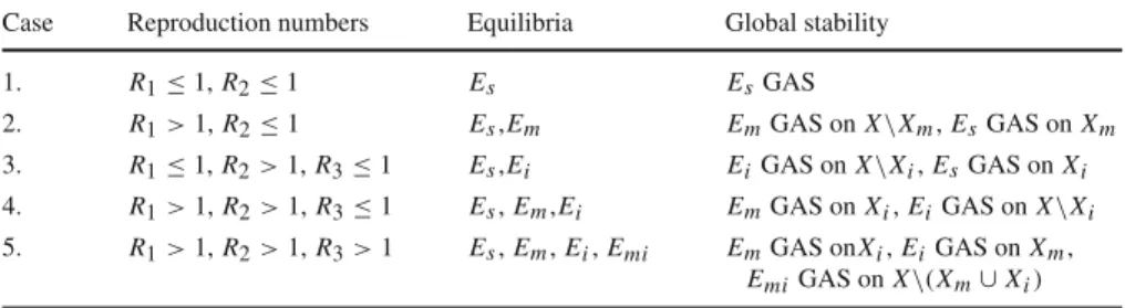
Table 1 Reproduction numbers, existing equilibria and global stability: the complete characterization of the dynamics
Case Reproduction numbers Equilibria Global stability
1. R1≤1,R2≤1 Es EsGAS
2. R1>1,R2≤1 Es,Em EmGAS onX\Xm,EsGAS onXm 3. R1≤1,R2>1,R3≤1 Es,Ei EiGAS onX\Xi,EsGAS onXi 4. R1>1,R2>1,R3≤1 Es,Em,Ei EmGAS onXi,EiGAS onX\Xi 5. R1>1,R2>1,R3>1 Es,Em,Ei,Emi EmGAS onXi,EiGAS onXm,
EmiGAS onX\(Xm∪Xi)
thus we obtain that the limit of solutions started in X\(Xm ∪Xi)is Emi. Solutions started inXm tend toEi.
The limit set of solutions of Eq. (6) started inXmis the equilibriumA
d,0 . Thus, in this case the equation forHm(t)on the limit set has the form (7). Similarly to the previous cases, the nontrivial solutions of this equation have the form
Hm(t)= Cγeγt
Cβ1eγt+γ forC∈R+.
We haveγ >0 if and only ifR1>1. Thus, forR1≤1,Hm(t)→0 (ast → ∞) and the limit of solutions started inXiisEs, while forR1>1 we obtain the solutions started inXitend toEmi. To complete the proof of the theorem, we notice thatR2>1 andR3>1 implyR1>1:
1<R2R3=R1 (d+δ)(d+α)
αδ+R2d(d+α+δ) <R1,
and for R1 >1 we already established the global asymptotic stability of Em onXi.
The proof of (iii) is complete.
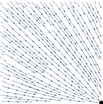
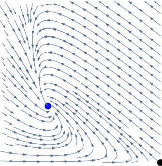
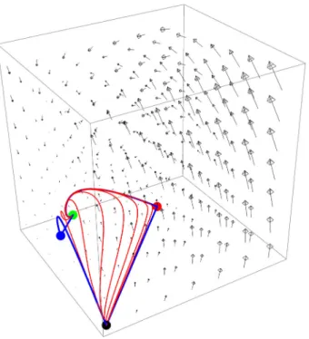
The results of Theorem 6.1 are summarized in Table 1. In Figs. 2, 3, 4, 5 and6, we denotedEs by black ,Emby red ,Ei by blue andEmiby green.
7 The two-dimensional subsystem of susceptible bees
In this section we consider the two-dimensional subsystem of (3) consisting of the first two equations and make a discussion about the equilibrium points, local and global stability. Also, we assume that the subsystem (4) is in a steady state, and substitute any of the equilibria of the subsystem (4) into these to obtain the two-dimensional system
Fig. 2 Case 1:R1 ≤1, R2 ≤ 1. Representation of the flow and the global attractor consisting of the equilibriumEs
Fig. 3 Case 2:R1 > 1,R2 ≤1. Representation of the flow and the global attractor consisting of the equilibriumEsandEm
Fig. 4 Case 3:R1≤1,R2>1 andR3≤1. Representation of the flow and the global attractor consisting of the equilibriaEsandEi
Fig. 5 Case 4:R1>1,R2>1 andR3≤1. Representation of the flow and the global attractor consisting of the equilibriaEs,Em,Eiand connecting orbits fromEstoEi
Fig. 6 Case 5:R1>1,R2>1 andR3>1. Representation of the flow and the global attractor consisting of the equilibriaEs,Em,Ei,Emiand connecting orbits fromEstoEmi
Hs(t)=L1−L2Hs(t)−
σ1−σ2
F s F s+H s
Hs(t) +
σ1−σ2
F s F s+H s
Fs(t)
Fs(t)=
σ1−σ2
F s F s+H s
Hs(t)−L2Fs(t)
−
σ1−σ2
F s F s+H s
Fs(t),
(9)
where
L1= A+αHm∗+αHi∗,
L2=d+β1Hm∗+β2Hi∗ (10) andHm∗ andHi∗are the second, resp. third coordinates in any of the four equilibria (5).
We calculate the equilibria of the subsystem (9) by solving the algebraic system of equations