Article
Density of Biogas Power Plants as An Indicator of Bioenergy Generated Transformation of
Agricultural Landscapes
Nandor Csikos1,*, Malte Schwanebeck2, Michael Kuhwald3 , Peter Szilassi1 and Rainer Duttmann3
1 Department of Physical Geography and Geoinformatics, University of Szeged, Egyetem u. 2–6, H-6722 Szeged, Hungary; toto@geo.u-szeged.hu
2 Department of Geography, Division of Physical Geography: Landscape Ecology and Geoinformation Science, Center for Geoinformation, Kiel University, D-24098 Kiel, Germany; mschwanebeck@gis.uni-kiel.de
3 Department of Geography, Division of Physical Geography: Landscape Ecology and Geoinformation Science, Kiel University, D-24098 Kiel, Germany; kuhwald@geographie.uni-kiel.de (M.K.);
duttmann@geographie.uni-kiel.de (R.D.)
* Correspondence: csikos@geo.u-szeged.hu
Received: 20 March 2019; Accepted: 24 April 2019; Published: 29 April 2019 Abstract:The increasing use of biogas, produced from energy crops like silage maize, is supposed to noticeably change the structures and patterns of agricultural landscapes in Europe. The main objective of our study is to quantify this assumed impact of intensive biogas production with the example of an agrarian landscape in Northern Germany. Therefore, we used three different datasets; Corine Land Cover (CLC), local agricultural statistics (Agrar-Struktur-Erhebung, ASE), and data on biogas power plants. Via kernel density analysis, we delineated impact zones which represent different levels of bioenergy-generated transformations of agrarian landscapes. We cross-checked the results by the analyses of the land cover and landscape pattern changes from 2000 to 2012 inside the impact zones. We found significant correlations between the installed electrical capacity (IC) and land cover changes. According to our findings, the landscape pattern of cropland—expressed via landscape metrics (mean patch size (MPS), total edge (TE), mean shape index (MSI), mean fractal dimension index (MFRACT)—increased and that of pastures decreased since the beginning of biogas production.
Moreover, our study indicates that the increasing number of biogas power plants in certain areas is accompanied with a continuous reduction in crop diversity and a homogenization of land use in the same areas. We found maximum degrees of land use homogenisation in areas with highest IC.
Our results show that a Kernel density map of the IC of biogas power plants might offer a suitable first indicator for monitoring and quantifying landscape change induced by biogas production.
Keywords: renewable energies; biogas power plants; silage maize; pasture; landscape metrics; land cover change; landscape diversity; agricultural diversity
1. Introduction
In order to lower greenhouse gas emissions, the EU member states intend to add an increasing share of renewable energy sources to their national energy systems. Renewable resources like wind, solar, geothermal, hydropower, and biogas produced from biomass allow the generation of electricity and heat, which contributes to reaching the climate protection goals of the European energy sector [1]. Currently, energy from biogas, mostly electricity [2], yields 7.6% of primary renewable energy production in the EU. Biogas produced by anaerobic co-digestion of waste and agricultural products like manure and energy crops contributes 69% to this share [3].
Sustainability2019,11, 2500; doi:10.3390/su11092500 www.mdpi.com/journal/sustainability
Today, the usage of biogas and biomass to produce electricity is a world-wide applied technology.
It is a relevant topic all over the world, as shown by the current studies on sustainable use of crop residues in biogas power plants in the USA [4], the changes in agriculture systems in East European countries [5,6], or analysis of straw and manure potentials as feedstock in China [7].
Especially in Germany, the introduction of a renewable energy law in 2000 and its amendments in 2004 and 2009 have encouraged a boost in biogas production. This law subsidizes electricity production from renewable energy resources, including biogas. At the time of its implementation, the law guaranteed comparatively high and constant feed-in tarifffor new biogas power plants over a 20-year period. It also introduced a bonus for the use of renewable substrate materials like manure and energy crops. For these reasons, a strong increase in the number and installed capacity of biogas power plants took place [8]. In 2014, Germany produced 50% of the total biogas among the EU member states [3]. Most of this biogas is used to generate electricity in more than 10,000 biogas power plants with an installed capacity of over 4500 MW [8], which are mainly operated by local farmers.
Agricultural residue like manure from cattle and pigs, and energy crops contribute to 97% of the biogas power plants’ feedstock, with silage maize (or green maize) (Zea mays L.) as the major crop source material for biogas production [3].
Silage maize for biogas purposes is currently grown on about 900,000 ha in Germany [9]. Younger amendments to the original renewable energy law in 2012 and 2014 slowed down the former rapid development of new biogas power plants [8]. However, several studies state that this energy policy instrument caused many changes in local agricultural systems in different regions of Germany [10–12].
These include changes in land-use [13,14], bio-diversity aspects like species composition [15,16], ecosystem services [17] and landscape structure and functions [18].
A central part in the discourse on the agricultural biogas production is the question of whether increased use of biogas for energy production leads to a loss of permanent pasture because of increased silage maize cultivation. Lükers-Jans et al. [13] postulate a triangle of mutually interacting input factors for this kind of land-use change driven by energy policy. They recommend a future investigation of the correlation between the installed capacity of biogas power plants and the expansion of both maize cultivation area and conversion of pastures. It has to be considered that the silage maize areas located in regions with high livestock density and the livestock density also shows correlation with the biogas power plants [13]. Higher installed electrical capacity means more manure and silage maize needed to feed the biogas power plants. Laggner et al. [14] noted an increase in silage maize area in most communities where pastureland area decreased between 1999 and 2007. Conversion of permanent pasture to grow crops like silage maize is related to increasing risks of soil erosion and compaction [19,20], increasing nitrogen mineralization and leaching [21–23], increasing release of greenhouse gases from humus degradation [22] and changes in local bio-diversity [16,18,22].
In addition, the traffic in the proximity to biogas power plants usually increases seasonally due to the large amount of feedstock material transported from the surrounding fields to the power plant site in harvesting time [24]. In Germany a high proportion of biogas power plants were built on already existing farms, instead of installing them on undeveloped land like in the Czech Republic and Italy [5,25].
Based on the maps of Schmidt [26], in Germany highest shares of silage maize area can be detected in the most northern federal-states of Schleswig-Holstein and Lower-Saxony between 1999 and 2013.
Using remote sensing, Oppelt et al. [27] examined a small catchment in Schleswig-Holstein, and detected local land-use changes that shifted from cereals and permanent pasture to increases in silage maize. They identified areas where intense conversion of pasture occurred over a 3-year period from 2009 to 2011.
Similar results were reported by Kandziora et al. [28] from the areas in the Central East and the North East of Schleswig-Holstein. Based satellite data they found a decrease in pastureland by about 50% from 1987 to 2007 and complementary increase in cropland at the same time. Areas cultivated with maize grew by 83% (Central East), respectively 249% (North East) over this timespan. Furthermore,
crop rotation analyses for the years 2009 to 2011 further showed conversion of pasture in combination with mono-cropping of maize.
Landscape metric parameters are widely used as indicators of biodiversity, water quality and land cover change [29–34] and they are still being further developed [35–37]. They offer a spatial tool set for analysing entire landscapes, as well as the arrangement and properties of their features.
These metrics, which originated from the landscape ecology discipline [38,39], can provide information about the richness, evenness or fragmentation of a landscapes via quantitative indices. They can indicate, illustrate and quantify the cumulative effects of small changes in land use-patterns, landscape structures and land cover diversity, as well as in landscape functions. Altogether landscape metrics provide quantitative measures for quantifying and monitoring landscape change [29,40–42].
Uuemaa et al. [30,31] stated that more studies should sharpen attention on the impacts of policy instruments on agricultural landscapes. Further, Lausche et al. [36] argued that land-use policies as well as the introduction of new technologies could have a considerable impact on landscape patterns.
Based on these contentions, this study focuses on quantifying land use and landscape change processes induced by the intensification of silage maize cultivation for biogas production. We hypothesize that landscape metrics and diversity indicators are suitable for monitoring the impacts of energy policies on the structure and diversity of agricultural landscapes, which are increasingly used for energy production.
To our knowledge no study exists that analyses the transformation of agricultural landscapes as a consequence of increasing biomass production, which utilizes landscape metrics and diversity indices calculated from readily available satellite and topographic data at regional scales. Therefore, the objectives of this study are:
(1) to delineate the zones of different level of impacts in terms of landscape change by biogas production in agrarian landscapes based on a density map of installed electrical capacity (IC) of the biogas power plants;
(2) to quantify the impact of biogas power plants via size- and shape- related landscape metrics as well as diversity indices and to investigate the statistical relationships between the IC of biogas power plants and the various metrics.
The main outcome of our study is that we can delineate different impact zones of landscape change based on the installed electrical capacity density of biogas power plants for a federal state in northern Germany. These areas are highly affected by biogas production. We analysed the distribution and changes of land use categories and landscape indices inside of the impact zones to show the usefulness of this method.
2. Materials and Methods
2.1. Study Area
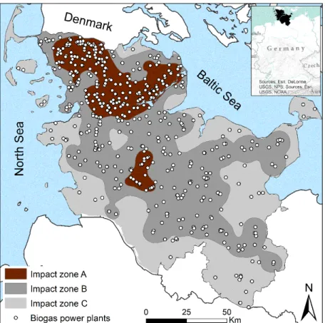
Schleswig-Holstein, the northernmost Federal State of Germany, serves as the study area. It is surrounded by the Baltic Sea in the east, Denmark to the north and the North Sea to the west (Figure1).
The climate is humid with a mean annual temperature of 8.6◦C and mean annual precipitation of 878 mm (weather station Schleswig, 1981–2010, [43]). Schleswig-Holstein has a high level of agricultural use: in 2016, 41.5% of the federal-state’s area was arable land, 20.7% pasture, 10.6% forest, 13.2% sealed area and 14% other land cover types [44].
Sustainability2019,11, 2500 4 of 23
Nations (FAO) [45]). The Young Moraine Hill Country is intensively used for crop production, mainly winter wheat (Triticum aestivum L.), barley (Hordeum vulgare L.) and oilseed rape (Brassica napus L.).
In contrast, the sandy deposits of the outwash plain (“Vorgeest” and “Hohe Geest”) are characterized by less fertile soils such as Podzols and podsolic Gleysols and frequently wetted Gleysols at deeper positions. While the latter are typically used as meadow and pastureland for livestock farming, the nutrient-poor and water-limited podzolic soils are traditionally cultivated with silage maize (Zea mays L.) and rye (Secale cereale L.) for livestock feeding. The Marshlands on the western part of Schleswig-Holstein have developed since the end of the last ice age. They consist mainly of fine- grained marine sediments with higher shares of silt and clay deposited by the North Sea during the Holocene sea level rise. The younger soils (Calceric Fluvisols/Gleysols) of the Marshlands are highly productive and dominantly used for winter wheat production. The older and frequently wet marshland soils provide less favourable conditions for arable farming and generally used only for pasture.
Figure 1. The federal state of Schleswig-Holstein in North Germany with main landscape units and biogas power plant sites.
2.2. Data Sources and Databases
Small-scale land cover and land-use data for the study site were extracted from the Corine Land Cover (CLC) project data. This data was used to calculate the landscape metric and land cover diversity parameters (Table 1). The CLC data sets are based on satellite image raster data and represent land cover and land-use in Europe at a scale of 1:100,000 at different years. They include 44 classes of land cover and land use, of which 37 are relevant for Germany [46]. A 25 ha minimum mapping unit is used to represent areal unities while linear land cover units are represented with a minimum width of 100 m [34,44,47]. In this study, CLC data sets for the years 2000 and 2012 were used, because the first biogas power plants were constructed around 2000 and subsequently increased strongly in number until at least 2012.
Statistical data from the German Agricultural Structure Survey (Agrar-Struktur-Erhebung, ASE) was used to calculate land cover and crop diversity metrics on municipality and landscape level (see Table 1). This statistical survey is conducted as a full census that gathers data on farm structures and land use as well. For the study region, results from the years 2003 and 2010 were available aggregated
Figure 1.The federal state of Schleswig-Holstein in North Germany with main landscape units and biogas power plant sites.
Based on the geological formations that developed during glacial and Holocene times, Schleswig-Holstein can be divided into four main landscapes from West to East: the “Marschlands”, the “Hohe Geest” representing the slightly elevated and eroded remains of terminal moraine tills of the penultimate glaciation (Saalian), the glacial outwash plain (“Vorgeest”), and the “Young moraine hill country” covering the eastern parts of Schleswig-Holstein. The Young Moraine Hill Country is characterized by glacial deposits of the Weichselian glaciation. Parent material for soil development mainly consists of sandy loamy to loamy textures, providing highly fertile soils, such as Luvisols, Cambisols and their stagnic subtypes (according to Food and Agriculture Organization of the United Nations (FAO) [45]). The Young Moraine Hill Country is intensively used for crop production, mainly winter wheat (Triticum aestivum L.), barley (Hordeum vulgare L.) and oilseed rape (Brassica napus L.).
In contrast, the sandy deposits of the outwash plain (“Vorgeest” and “Hohe Geest”) are characterized by less fertile soils such as Podzols and podsolic Gleysols and frequently wetted Gleysols at deeper positions. While the latter are typically used as meadow and pastureland for livestock farming, the nutrient-poor and water-limited podzolic soils are traditionally cultivated with silage maize (Zea mays L.) and rye (Secale cereale L.) for livestock feeding. The Marshlands on the western part of Schleswig-Holstein have developed since the end of the last ice age. They consist mainly of fine-grained marine sediments with higher shares of silt and clay deposited by the North Sea during the Holocene sea level rise. The younger soils (Calceric Fluvisols/Gleysols) of the Marshlands are highly productive and dominantly used for winter wheat production. The older and frequently wet marshland soils provide less favourable conditions for arable farming and generally used only for pasture.
2.2. Data Sources and Databases
Small-scale land cover and land-use data for the study site were extracted from the Corine Land Cover (CLC) project data. This data was used to calculate the landscape metric and land cover diversity parameters (Table1). The CLC data sets are based on satellite image raster data and represent land cover and land-use in Europe at a scale of 1:100,000 at different years. They include 44 classes of land
cover and land use, of which 37 are relevant for Germany [46]. A 25 ha minimum mapping unit is used to represent areal unities while linear land cover units are represented with a minimum width of 100 m [34,44,47]. In this study, CLC data sets for the years 2000 and 2012 were used, because the first biogas power plants were constructed around 2000 and subsequently increased strongly in number until at least 2012.
Table 1.Data sources used in this study (based on [48–50]).
Corine Land Cover (CLC)
Agricultural Structure Survey
(ASE) Biogas Power Plants
Scale 1: 100,000
(>25 ha) Municipality level (local scale) Coordinates of power plant site Nomenclature 44 classes,
37 relevant in Germany
Every types of agricultural plants and animals
Used time scales 2000, 2012 2003, 2010 2014
Coverage Europe Schleswig-Holstein (Germany) Schleswig-Holstein
(Germany) Source Federal Statistical Office Federal Statistical Office Federal-state office
Statistical data from the German Agricultural Structure Survey (Agrar-Struktur-Erhebung, ASE) was used to calculate land cover and crop diversity metrics on municipality and landscape level (see Table1). This statistical survey is conducted as a full census that gathers data on farm structures and land use as well. For the study region, results from the years 2003 and 2010 were available aggregated at municipality (1106 municipality in Schleswig-Holstein) and at landscape level, provided by the statistical authority. For calculating diversity metrics, the hectares of land-use for crops and pasture were joined to official municipality geodata inside the study area [44].
Data on the location and installed electrical capacity (IC) of biogas power plants in Schleswig-Holstein were provided by the State Office for Agriculture Environment and Rural Spaces [48]. The dataset used in this study gives information on 925 sites of biogas power plants from the year 2014 (Figure1), including the characteristics of the generators used to produce electricity from biogas.
We used these three different datasets from five different years as, they are not available for the same year.
2.3. Landscape Metrics
Landscape metric parameters are important quantitative implements in landscape ecology [51].
The selection of area and shape related landscape metrics used in this work (see below), is based on the work of Szabó[52] and Walz [51]. The software developed by Lang and Tiede [53] was employed for the calculation of landscape metrics. Concerning pattern analyses (e.g., [54–57]), this study uses parameters that are suited to indicate temporal changes in area, structure and diversity at the landscape and patch level (for more details see TableA1). Patch level metrics, created for individual land cover patches, characterize the spatial character and context of patches. These patch metrics serve primarily as the computational basis for developing a landscape metric. Class level metrics unify the patches of a given land cover type (class). Landscape level metrics are integrated over all patch types or classes over the full extent of the data. Like class metrics, they may be integrated by a simple or weighted averaging, or may reflect aggregate properties of the patch mosaic.
As many of the available measures of landscape metrics are partially or completely redundant, such as patch density (PD) and mean patch size (MPS), only the MPS was considered in this study.
The MPS has been widely applied in landscape monitoring, since it is commonly agreed that the occurrence and abundance of different kinds of species and species richness as well, strongly correlates with the patch size. Amongst patch size metrics, edge-metrics can be used to characterize the spatial grain and the structural variety of a landscape [39]. The total edge (TE) of all patches in a selected
landscape is known to have several effects on ecological phenomena [30]. Both of the landscape indicators, MPS and TE, were used to represent the continuity of the landscape’s structure during the observed period from 2000 to 2012. The Mean Shape Index (MSI) was calculated to further describe the changes in the geometrical complexity of a patches. The mean fractal dimension index (MFRACT) is a normalized shape index in which the perimeter and area are log transformed [39].
For evaluating changes in landscape and in structural richness, the Shannon diversity (SDI), evenness (SEI) and the richness indexes (RI) according to Uuemaa et al. [30] were applied, involving all land use classes in the study area.
To assess the effects of the increasing number of biogas power plants on the landscape patterns’
grain size, MPS and TE have been chosen. The effects on the shape complexity of the individual land use types were quantified by using MSI and MFRACT as indicators. We used the area weighted mean (AWM) values of these indices in the statistical calculations. AWM equals the sum of all patches in the area, of the corresponding patch type multiplied by the proportional abundance of the patch and divided by the sum of the patch areas.
2.4. Spatial and Statistical Analysis
In order to relate the changes in land cover and land cover pattern to the IC of biogas power plants inside an area we delineated three impact zones of different density of IC (MW km−2) using Kernel Density calculation within ArcGIS 10.3 software [58]. Separation of the single IC density classes followed the Jenks natural breaks classification method [59]. In detail, three impact zones were defined:
“impact zone A” (1.03 to 2.46 MW km2), “impact zone B” (0.3 to 1.03 MW km2), and “impact zone C”
(<0.3 MW km2) (Figure2).
Sustainability 2019, 11, x FOR PEER REVIEW 7 of 24
impact zone B = 0.3–1.03 MW/km2, impact zone C = 0–0.3 MW/km2. Impact zone A is mainly located in the central northern part of Schleswig-Holstein, which is traditionally used for livestock- breeding and milk production. Areas of impact zone B comprise nearly all the interior landscapes, while impact zone C areas occur along the periphery of the federal state.
Figure 2. Biogas generated landscape transformation impact zones in the study area based on the Kernel density of installed capacity of biogas power plants: impact zone A = 1.03–2.46 MW/km2, impact zone B = 0.3–1.03 MW/km2, impact zone C = 0–0.3 MW/km2 (data source: Agriculture Environment and Rural Spaces 2014 [48]).
3.2. Validation of the Delineated Impact Zones
3.2.1. Land Cover Changes Inside the Impact Zones
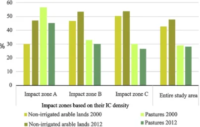
Based on the CLC data sets from 2002 and 2012 various changes regarding land use can be detected, in the entire study area. The biggest changes relate to the CLC class “non-irrigated arable land” and “pastures” inside the delineated impact zones. According to Bossard et al. [47], the land use class "non-irrigated arable land" refers to land parcels cultivated with annually harvested non- permanent crops, usually grown in a crop rotation. The land use class “pasture” subsumes all permanent grassland characterized by agricultural use, like grazing or harvesting of grass. Regarding the entire study area, the amount of arable land increased by 5%, while the pasture decreased by 1%.
Between 2000 and 2012, impact zone A reveals an increase of "non-irrigated arable land” by 17% and a decrease in pasture area by 11%. Inside impact zones B and C, only small changes of a few percent were registered (Figure A1).
Based on the ASE dataset, we analysed the changes in different agricultural land use types for the entire study area. Figure 3 shows the changes in silage maize and pastures area. These land use types experienced the greatest change from 2003 to 2010 (Figure 3). The Pasture area decreased by 68,000 hectares, while the silage maize acreage increased by 89,000 hectares.
Figure 2. Biogas generated landscape transformation impact zones in the study area based on the Kernel density of installed capacity of biogas power plants: impact zone A=1.03–2.46 MW/km2, impact zone B=0.3–1.03 MW/km2, impact zone C=0–0.3 MW/km2(data source: Agriculture Environment and Rural Spaces 2014 [48]).
The structural characteristics of land cover and the land cover pattern inside of these impact zones and their changes were analysed using the CLC data sets. AWM values have been calculated based on the class level landscape indices in the three impact zones and in the total study area using the Geospatial Modelling Environment [60]. This tool uses just the patches which having their centroids inside a given impact zone. Area-weighted metrics are more meaningful in ecology than the means as suggested by Gustafson [61]. Based on CLC data, the area-weighted size (AWMPS), edge (AWMTE) and shape metrics (AWMFRACT, AWMSI) were calculated for the landscape level and the class level (classes are patches of “arable land” and “pastures”) considering the individual impact zones and the entire federal-state of Schleswig-Holstein. CLC data sets were also used to calculate the landscape level diversity indices (SDI, SEI and RI) for the three impact zones of the study area. The same indices have been calculated for the municipality level using the ASE data set to detect changes in agricultural diversity (all kinds of agricultural land use) and crop diversity (only crop types) at local scale.
The landscape metrics related to size and shape (AWMPS, AWMTE, AWMFRACT) were calculated using the V-Late 2.0 (Vector-based Landscape analysis tool extension of ArcGIS 10.2) tool [53]. The same applies for the land cover diversity indices (SDI, SEI, RI) derived from CLC data. For calculating the same agricultural diversity indices from the ASE data-set, a Microsoft Excel add-in [62] has been applied. We calculated the area weighted shape and size related landscape indices, and the averages of the land cover and crop diversity indices for each municipality of the study area. We counted and summarized every biogas power plants and their IC (MW) in every municipality. At the statistical analysis part of the work, we selected the municipalities (containing the metrics and IC values) inside every impact zone and calculated the coefficient value for every impact zone. We ran a one-way analysis of variance (ANOVA) test on our municipality dataset (containing the landscape metrics and diversity indices). This analysis can be performed on a dataset with three or more groups, so the three impact zones were declared as groups. The ANOVA test is a technique to compare the means of groups using F distribution. The null hypothesis is that samples in all groups are drawn with the same mean values. We used the Tukey post hoc multiple comparison, which shows, which groups differed from each other. For statistical analyses between the IC of biogas power plants, and the landscape indices describing the shape and size characteristics of land cover patches, and the land cover diversity, the non-parametric Spearman rank correlation was used. IBM SPSS Statistics 22 software [63] was used for statistical evaluation.
3. Results
3.1. Delineation of the Bioenergy Impact Zones
Kernel density calculation enabled the separation of three impact zones of different density of IC of biogas power plants (Figure2). We named the three delineated impact zones based on the density of biogas power plants’ installed electrical capacity: impact zone A=1.03–2.46 MW/km2, impact zone B=0.3–1.03 MW/km2, impact zone C=0–0.3 MW/km2. Impact zone A is mainly located in the central northern part of Schleswig-Holstein, which is traditionally used for livestock- breeding and milk production. Areas of impact zone B comprise nearly all the interior landscapes, while impact zone C areas occur along the periphery of the federal state.
3.2. Validation of the Delineated Impact Zones
3.2.1. Land Cover Changes Inside the Impact Zones
Based on the CLC data sets from 2002 and 2012 various changes regarding land use can be detected, in the entire study area. The biggest changes relate to the CLC class “non-irrigated arable land” and
“pastures” inside the delineated impact zones. According to Bossard et al. [47], the land use class
"non-irrigated arable land" refers to land parcels cultivated with annually harvested non-permanent crops, usually grown in a crop rotation. The land use class “pasture” subsumes all permanent grassland
characterized by agricultural use, like grazing or harvesting of grass. Regarding the entire study area, the amount of arable land increased by 5%, while the pasture decreased by 1%. Between 2000 and 2012, impact zone A reveals an increase of "non-irrigated arable land” by 17% and a decrease in pasture area by 11%. Inside impact zones B and C, only small changes of a few percent were registered (FigureA1).
Based on the ASE dataset, we analysed the changes in different agricultural land use types for the entire study area. Figure3shows the changes in silage maize and pastures area. These land use types experienced the greatest change from 2003 to 2010 (Figure3). The Pasture area decreased by 68,000 hectares, while the silage maize acreage increased by 89,000 hectares.Sustainability 2019, 11, x FOR PEER REVIEW 8 of 24
Figure 3. Area changes of the different agricultural land use types in federal state of Schleswig- Holstein, based on the German Agricultural Structure Survey (Agrar-Struktur-Erhebung, ASE) 2003 and 2010 datasets.
Correlating the ASE data to the impact zones shows that the proportion of silage maize area strongly increased, mainly inside impact zone A. In some municipalities, the proportion of silage maize amounts to 66% of the total area of agricultural land use (Figure 4).
(a) (b)
Figure 4. The proportion of silage maize areas at municipality level, based on ASE database in 2003 (a) and in 2010 (b).
Compared to the entire state of Schleswig-Holstein, where the silage maize acreage increased on average 9% between 2003 and 2010, impact zone A shows a stronger positive change in silage maize acreage of about 20%. During the same period, the pasture area decreased by the same percentage.
The biggest changes in land use appear in the northern parts of the glacial outwash plain (Vorgeest).
In contrast, only modest changes occurred in the impact zones C (comparing Figure 4a and Figure Figure 3.Area changes of the different agricultural land use types in federal state of Schleswig-Holstein, based on the German Agricultural Structure Survey (Agrar-Struktur-Erhebung, ASE) 2003 and 2010 datasets.
Correlating the ASE data to the impact zones shows that the proportion of silage maize area strongly increased, mainly inside impact zone A. In some municipalities, the proportion of silage maize amounts to 66% of the total area of agricultural land use (Figure4).
Sustainability 2019, 11, x FOR PEER REVIEW 8 of 24
Figure 3. Area changes of the different agricultural land use types in federal state of Schleswig- Holstein, based on the German Agricultural Structure Survey (Agrar-Struktur-Erhebung, ASE) 2003 and 2010 datasets.
Correlating the ASE data to the impact zones shows that the proportion of silage maize area strongly increased, mainly inside impact zone A. In some municipalities, the proportion of silage maize amounts to 66% of the total area of agricultural land use (Figure 4).
(a) (b)
Figure 4. The proportion of silage maize areas at municipality level, based on ASE database in 2003 (a) and in 2010 (b).
Compared to the entire state of Schleswig-Holstein, where the silage maize acreage increased on average 9% between 2003 and 2010, impact zone A shows a stronger positive change in silage maize acreage of about 20%. During the same period, the pasture area decreased by the same percentage.
The biggest changes in land use appear in the northern parts of the glacial outwash plain (Vorgeest).
In contrast, only modest changes occurred in the impact zones C (comparing Figure 4a and Figure Figure 4.The proportion of silage maize areas at municipality level, based on ASE database in 2003 (a) and in 2010 (b).
Compared to the entire state of Schleswig-Holstein, where the silage maize acreage increased on average 9% between 2003 and 2010, impact zone A shows a stronger positive change in silage maize acreage of about 20%. During the same period, the pasture area decreased by the same percentage.
The biggest changes in land use appear in the northern parts of the glacial outwash plain (Vorgeest). In contrast, only modest changes occurred in the impact zones C (comparing Figure4a,b). Furthermore, the ASE data indicate that a large proportion of pasture had been transformed into arable land for silage maize production (FigureA2).
3.2.2. Landscape Metrics Inside the Impact Zones
The effects of increased biogas production on the spatial structures of “non-irrigated arable land”
and “pasture” were quantified via a set of area, edge and shape related landscape metrics calculated from CLC data. In general, FigureA3reveals decreases in size (AWMPS), perimeter (AWMTE) and complexity (AWMSI, AWMFRACT) for the arable land and pastures compared to state wide conditions.
Further, the data for impact zone A deviate noticeably from the others. Here, the edge length indicator AWMTE and the complexity indicators AWMSI and AWMFRACT of arable land increased from 2000 to 2012. In contrast, the same indicators for pasture areas show a strong decrease. The patch sizes (AWMPS) of pastures also declined drastically during this period. These findings suggest that patches occupied by cropland became bigger and more complex, while the perimeters of these patches increased relative to area they enclose. For pastureland the opposite trend occurred, as patches became smaller and more compact. Except for the AWMFRACT, which shows an increase for arable land and pastures in the impact zone B and C, all other shape and size related patch level metrics reveal declining values.
3.2.3. Land Cover Diversity Inside the Impact Zones
Land cover diversity indices (RI, SDI and SEI) were calculated from CLC data. They show a decreasing tendency between 2000 and 2012 inside the entire study area. The strongest decline can be observed for the SDI which decreased from 1.207 to 1.067. Furthermore, the SEI changed from 0.403 to 0.356 (TableA2). Impact zone A is characterized by the smallest SDI and SEI numbers, while the RI does not reflect any changes in these areas.
Moreover, ASE statistics indicate a strong decline in agricultural and crop diversity. The richness index (RI) calculated for agricultural diversity decreased in the individual impact zones as well as in the entire area of the federal state of Schleswig-Holstein (Table2). Strongest reductions of RI occurred in areas of impact zone A, which also revealed the largest negative changes in SDI, while the SEI only varied slightly (Table2).
Table 2.Changes in the diversity indices between 2003 and 2010 for different agricultural land use and crop types based on ASE 2003 and 2010 data sets (IC=Installed electrical Capacity).
Landscape Diversity Indices
Impact Zones Based on Their IC Density Entire Study Impact Zone A Impact Zone B Impact Zone C Area
Agricultural diversity
Richness −4.543 −4.009 −3.377 −3.849
Shannon Diversity −0.642 −0.56 −0.478 −0.541
Shannon Evenness −0.012 −0.014 −0.031 −0.019
Crop diversity
Richness −1.718 −1.359 −0.955 −1.261
Shannon Diversity −0.509 −0.359 −0.241 −0.337
Shannon Evenness −0.266 −0.144 −0.091 −0.142
For crop diversity areas of impact zone A show the strongest change, compared to the entire study area as well as to the impact zones B and C.
3.2.4. Link between Installed Electrical Capacity (IC) and Changes in Land Use and Landscape Indices in the Impact Zones
There was a statistically significant difference between groups as determined by one-way ANOVA test, non-irrigated arable land: AWMPS (F (2, 1087)=27,p=3.57−12), AWMTE (F (2, 1087)=25.6, p=1.35−11), AWMSI (F (2, 1087)=10.89,p=2.07−5), AWMFRACT (F (2, 1087)=0.15,p=0.6) (TablesA3 andA4); pastures land: AWMPS (F (2, 1087)=5.94,p=0.003), AWMTE (F (2, 1087)=5.66,p=0.004), AWMSI (F (2, 1087)=5.42,p=0.005), AWMFRACT (F (2, 1087)=4.71,p=0.009) (TablesA5andA6).
According to these results of the ANOVA test, the three delineated impact zone show significant difference in the mean of the landscape indices. The non-irrigated arable land patches’ shape and size characteristics show a significant positive correlation (p<0.05) with the IC of each impact zones and the entire area of Schleswig-Holstein, while the same landscape indices for the pasture land cover patches are negatively (but not significantly) correlated with IC. We used just the municipality dataset with IC and ASE data for this calculation.
The tightest positive significant correlations (p<0.01) between IC and AWMPS, AWMTE and AWMSI were measured in case of the “non-irrigated arable land use” patches located inside the impact zone A, while AWMFRACT only shows a weaker, but still significant correlation. Significant positive correlation coefficients were observed at the AWMSI of arable land, while negative coefficients were registered for AWMFRACT (r=−0.250,p<0.05) related to pasture land (Table3).
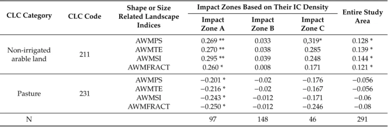
Table 3.Correlations between the IC and the landscape indices of impact zones based on the Corine Land Cover (CLC) 2012 database (IC=Installed electrical Capacity, AWMPS=Area weighted mean patch size, AWMTE=Area weighted mean total edge, AWMSI=Area weighted mean shape index, AWMFRACT=Area weighted mean fractal dimension index).
CLC Category CLC Code
Shape or Size Related Landscape
Indices
Impact Zones Based on Their IC Density
Entire Study Impact Area
Zone A
Impact Zone B
Impact Zone C
Non-irrigated
arable land 211
AWMPS 0.269 ** 0.033 0,319* 0.128 *
AWMTE 0.270 ** 0.038 0.285 0.139 *
AWMSI 0.295 ** 0.039 0.248 0.144 *
AWMFRACT 0.260 * 0.008 0.171 0.121 *
Pasture 231
AWMPS −0.201 * −0.02 −0.176 −0.056
AWMTE −0.216 * −0.02 −0.167 −0.056
AWMSI −0.243 * −0.012 −0.171 −0.06
AWMFRACT −0.250 * −0.012 −0.246 −0.08
N 97 148 46 291
**=Correlation is significant atp<0.01 level (2-tailed); *=Correlation is significant at thep<0.05 level (2-tailed).
Inside impact zone C, only the AWMPS yields a significant correlation (r=0.319,p<0.05) for arable land use. Inside impact zone B, no significant correlation was found between IC and the single indices.
Based on the ASE dataset we found significant correlations between the different types of agricultural land use and the installed capacity of biogas power plants (Table4). Silage maize acreage strongly positively correlates (r=0.572,p<0.01) with the IC density of the study area as well as with the individual impact zones (p<0.01). Significant correlations were calculated for regions of highest biogas production, while correlations get weaker with a decrease in IC density.
There was a statistically significant difference between groups as determined by one-way ANOVA test, SDI (F (2, 1108)=26.62,p=5.09−12), SEI (F (2, 1108)=14,p=9.98−7), RI (F (2, 1108)=20.63, p=1.6−9) (see TablesA7andA8). Based on the ANOVA test the mean values of the diversity indices in the impact zones show significant differences. Finally, significant inverse correlations between the IC of the impact zones and land cover diversity (SDI, RI SEI) can be determined (Table5). Impact zone A shows negative correlation coefficients with the diversity indices, SDI (r=−0,234,p<0.01), SEI (r=−0.257,p<0.01) and RI (r=−0.297,p<0.01). Impact zone C does not correlate with the individual
diversity indices. The findings in Table5suggest a decreasing influence of biogas production on landscape diversity with the decline of IC in a region.
Table 4.Correlations between the IC and different crop types in municipality level, based on Agricultural Statistical Survey 2010 (IC=Installed electrical Capacity).
Land Cover Types Impact Zones Based on Their IC Density Total Study Area Impact Zone A Impact Zone B Impact Zone C
Total agricultural areas 0.562 ** 0.428 ** 0.183 ** 0.397 **
Arable lands 0.541 ** 0.394 ** 0.152 ** 0.365 **
Silage maize 0.572 ** 0.389 ** 0.238 ** 0.462 **
Pasture 0.457 ** 0.242 ** 0.177 ** 0.339 **
Rye 0.254 ** 0.194 ** 0.013 0.196 **
Fallow 0.216 ** 0.153 ** 0.082 0.108 **
Wheat 0.182 * 0.235 ** 0.133 ** 0.137 **
Winter wheat 0.178 * 0.242 ** 0.158 ** 0.145 **
Barley 0.097 0.140 ** 0.123 * 0.085 **
Potato 0.086 0.128 ** 0.064 0.054
Winter rape 0.185 * 0.217 ** 0.115* 0.119**
Triticale 0.138 0.080 0.170 ** 0.076 *
N 160 544 408 1112
**=Correlation is significant atp<0.01 level (2-tailed); *=Correlation is significant at thep<0.05 level (2-tailed).
Table 5. Correlation between changes in crop diversity and the Installed electrical Capacity (IC) of biogas power plants, based on ASE.
Land Cover Diversity Indices Impact Zones Based on Their IC Density
Entire Study Area Impact Zone A Impact Zone B Impact Zone C
Richness Index −0.297 ** −0.228 ** −0.094 −0.241 **
Shannon Diversity Index −0.234 ** −0.098 * −0.029 −0.137 **
Shannon Evenness Index −0.257 ** −0.011 0.02 −0.019
N 160 544 408 1112
**=Correlation is significant atp<0.01 level (2-tailed); *=Correlation is significant at thep<0.05 level (2-tailed).
4. Discussion
4.1. Comparative Analyses of the Bioenergy Impact Zones
The existing biogas power plants (419 MW installed electrical capacity) in 2014 according to Melund [64] are mostly concentrated in the central and north-western glacial outwash plain of Schleswig-Holstein (see Figure 1), where soils of relatively poor quality dominate and there is a relatively high livestock density. The intensive use of biogas power plants in this area is offering a profitable additional or alternative income to farmers, compared to other common local land-use practices like permanent pasture for dairy farming fodder production. In addition, biogas power plants provide opportunities to process manure, which is available in large amounts in regions of high cattle density [10,14,22,23,65].
In many cases, fields that were formerly farmed with a diverse crop rotation today possess higher shares of silage maize, especially when they are located in the vicinity of biogas power plants in order to reduce transportation distances and to optimize economic production chains for biomass use [10,13,24,66]. Nevertheless, whether one can directly link locally observed trends of decreasing grassland area and simultaneously increasing silage maize acreage, energy production from biogas is still under discussion. Lüker-Jans et al. [13] investigated the relation between the expansion of silage maize area, conversion of pasture to arable land and the distance to existing biogas power plants for the Federal State of Hesse in Central Germany, using statistical and farm specific data sets
aggregated on municipality level. They found a significant correlation between existing and additional maize area and the distance to biogas power plants and a relationship between the vicinity of biogas power plants and conversion of pasture but also high correlation between existing maize area and livestock density. The proportion of silage maize increased in the entire study area from the beginning of 2000s (FigureA2), and based on the Figure3it increased by around 90,000 ha, while the pastures had a decrease around 70,000 ha. Figure4shows the municipalities where the increase was the highest and the silage maize maximum proportion reached the 66%. The expansion of the silage maize was most dynamic in the impact zone A. One can say that silage maize is probably the most significant indicator of the bioenergy generated transformation of the agricultural landscape.
The area of silage maize reveals a positive correlation (r=0.572;p<0.01) with the IC of biogas power plants and the strongest correlation compared to all other types of agricultural land use and arable crops (Table 4). The decrease in pasture area coincides with the start of increased silage maize growing. According to the ASE data set other crop and land use types did not increase to that proportion as silage maize did. For a small catchment in Germany Kandziora et al. [28] could prove the same results that the pasture area decreased to 50% from 1987 to 2007. The statistical analysis in our study make obvious that the silage maize acreage as well as the area of arable land (r=0.541) and pasture (r=0.457) significantly correlate (p<0.01) with the density of IC (Table4). Silage maize is the most common crop used for feeding the fermentation tanks. Interestingly, we found that the pasture area also positively correlates with IC. One reason might be that the farmers use the sown grass as a substrate for biogas production. According to Auburger et al. [67], the harvesting of pastures for biogas power plants could be an alternative way to replace silage maize to a limited degree, however this process is more expensive, so that farmers usually prefer the use of silage maize and manure for biogas production.
4.2. Statistical Analysis of the Landscape Metric Parameters in the Bioenergy Impact Zones
Comparing the two CLC data sets from 2000 and 2012 reveals that the patches of arable lands became larger and complex, while the patches covered with pasture became more compact, including a reduced length of their margins/edges. This holds especially true for those regions that have a high density of installed biogas power plants. These findings indicate that a higher percentage of arable fields become interconnected, grow in size and become more complex in shape, while a lesser number of isolated patches of pasture remains (FigureA3). These results fit to the work of Leuschner et al. [65], who showed for Schleswig-Holstein that from 1950 on the arable lands - and in the last decade the silage maize fields - were getting bigger with a more complex shape, while pastures were getting smaller, more fragmented and isolated.
As shown for the arable land located in the impact zone A, the AWMSI needs to be carefully interpreted and not decoupled from other indices, such as the AWMPS or AWMTE. A higher degree of compactness is not necessarily equivalent to a decrease in patch size or a reduction of edge lengths.
The situation mainly depends on the shape of the patches. In arable land patches with noticeable increases in AWMTE and also in complexity as indicated by AWMFRACT (FigureA3), the degree of compactness can also increase, for example, when the field plots are expanded to all sides and have more or less equal widths and length ratios.
The significant positive correlation between the IC and the area of arable land in impact zone A occurs because of the higher demand for silage maize, which is associated with increases in patch size and complexity within the landscape. In contrast, all landscape metrics indicators calculated for the pasture land use type reveal a significant inverse correlation with biogas production intensity. In the case of arable land, the AWMSI shows highest correlation with the IC density of biogas power plants, suggesting that an increase in IC, mainly affects the shape and complexity of the cropland patches.
From the indices derived for pasture land, the MFRACT is most strongly correlated to IC inside the impact zone A, implying that the intensity of biogas production contributes mainly to the form of patches, coupled with a higher fractioning of grassland patches, as indicated by the negative significant
correlation between AWMSI and IC density. In the impact zone A the AWMSI and AWMFRACT could be an indicator of the bioenergy generated transformation of agricultural landscapes, and they could help identify of this transformation. Uuemaa et al. [31] found that these are the most relevant metrics to describe landscape complexity and fragmentation, also for effect on species diversity.
4.3. Land Cover Diversity Changes in the Bioenergy Impact Zones
Land cover diversity indices were calculated from the CLC and ASE datasets, and we used the three most common diversity indices [68]. Regarding changes in landscapes and agricultural diversity, the RI index negatively and significantly correlated to the intensity of biogas production, and compared to all other diversity indices it has the highest negative correlation coefficient. The correlation between the RI and the IC density of biogas power plants is significant (r=−0.297,p<0.01, Table5), suggesting the RI to be a suited indicator to identify the bioenergy generated transformation in agricultural used areas [13,16].
Calculation based on CLC data shows the smallest values for SDI in the impact zone A and the strongest decrease of RI compared to the other regions (Table5). The same correlation holds true for SDI, indicating an increase in unevenness related of the different land use classes and crop types, as arable land is increasingly used for silage maize growing at a higher area percentage, including a higher share of maize monoculture. These support the knowledge from regional studies concerning the recent development in “energy landscapes” of Schleswig-Holstein, stating biogas production as the main driver of the landscape and land use change (e.g., [19,69]).
A decreasing trend in agricultural land cover diversity can be demonstrated by comparing the ASE data from 2003 and 2010, where most of the biogas power plants were newly constructed.
As already described for the CLC data set, the strongest decline in SDI and SEI numbers goes along with the increase in IC density, where the smallest numbers of these indicators are typical for those regions with the highest densities of biogas generated electricity (TableA2). Regarding the arable land, however, there is a strong increase in the proportion of silage maize, while other agricultural land use types changed by a few percent. Considering crop diversity, a negative change of SDI, SEI and RI can be observed for all impact zones, with the strongest decline occurring in the impact zone A (Table2). This indicates that the increase in silage maize production subsequently replaces other crops originally grown in these landscapes to a higher degree, which contributes to a loss of crop diversity and a depletion of landscape diversity. These results fit to the work of Jerrentrup et al. [70].
In order to prevent the undesired effects of land cover pattern change and landscape diversity decrease caused by the bioenergy-generated transformation of agricultural landscapes, landscape metrics and diversity indicators generated from data of various spatial scales can support a well-informed approach to landscape management. As shown in this study, spatial landscape metrics and diversity indicators are suited to spatially detect changes in land cover and crop diversity and in the landscape’s structure. In this example, landscape metrics have demonstrated that an uncontrolled bioenergy-generated transformation (expansion of maize cropping) may negatively affect landscape diversity.
5. Conclusions
This study shows that changes in land use, land cover pattern and landscape diversity caused by a bioenergy-driven transformation of agricultural landscapes can be identified via landscape metrics and diversity indicators applied to readily available data with different degrees of spatial and thematic aggregations. It reveals that the fostered production of electrical energy by biogas power plants can negatively affect the sizes and shapes of former pasture lands and increases the area, size and complexity of arable land patches. Moreover, for the study area in Northern Germany, the application of a Kernel density analysis based on data on the installed electrical capacity (IC) of biogas power plants could spatially identify the main impact zones (hot spots) of biogas energy generated declining land cover and crop diversity. Furthermore, this study provides quantified data on the spatio-temporal changes in landscape metrics indicators related to the different intensity zones of bioenergy generated landscape
transformation. According to our findings, the Kernel density map of the electrical capacity of biogas power plants are representing the impact zones of the biogas energy introduction. The calculations based on the Corine Land Cover database can be replicated in the countries of the European Union, where the CLC database exist, but other land cover or land use dataset can be adapting. The GIS tools used, released under general public licence (GPL), therefore are free to use for anyone, with the exception of Environmental Systems Research Institute (ESRI) ArcGIS, which is proprietary. The quality of calculated outcomes could be improved with the availability of remote sensing data of higher spatial and spectral resolution, and of a higher recovery rate, enabling a more detailed classification of land use and crop type, as shown by, for example, Kuhwald et al. [71].
Author Contributions:Conceptualization, N.C., M.S., M.K., P.S. and R.D.; Formal analysis, N.C.; Methodology, N.C., P.S.; Resources, M.S.; Supervision, P.S. and R.D.; Visualization, N.C. and M.S.; Writing—original draft, N.C.
and M.S.; Writing—review & editing, M.K., P.S. and R.D.
Funding: The Deutsche Bundesstiftung Umwelt MOE Scholarship Program founded N.C. We acknowledge financial support by Land Schleswig-Holstein within the funding programme Open Access Publikationsfonds.
Acknowledgments:We express our sincere thanks to James Petersen (Texas State University) for lingual editing an early draft and to Kilian Etter (Kiel University) for lingual editing the manuscript. We thank the anonymous referees for their valuable recommendations and suggestions.
Conflicts of Interest:The authors declare no conflict of interest.
Appendix A Appendix
Sustainability 2019, 11, x FOR PEER REVIEW 14 of 24
spatio-temporal changes in landscape metrics indicators related to the different intensity zones of bioenergy generated landscape transformation. According to our findings, the Kernel density map of the electrical capacity of biogas power plants are representing the impact zones of the biogas energy introduction. The calculations based on the Corine Land Cover database can be replicated in the countries of the European Union, where the CLC database exist, but other land cover or land use dataset can be adapting. The GIS tools used, released under general public licence (GPL), therefore are free to use for anyone, with the exception of Environmental Systems Research Institute (ESRI) ArcGIS, which is proprietary. The quality of calculated outcomes could be improved with the availability of remote sensing data of higher spatial and spectral resolution, and of a higher recovery rate, enabling a more detailed classification of land use and crop type, as shown by, for example, Kuhwald et al. [71].
Author Contributions: Conceptualization, N. C., M. S., M. K., P. S. and R. D.; Formal analysis, N. C.;
Methodology, N. C., P. S.; Resources, M. S.; Supervision, P. S. and R. D.; Visualization, N. C. and M. S.; Writing—
original draft, N. C. and M. S.; Writing—review & editing, M. K., P. S. and R. D.
Funding: The Deutsche Bundesstiftung Umwelt MOE Scholarship Program founded N.C. We acknowledge financial support by Land Schleswig-Holstein within the funding programme Open Access Publikationsfonds.
Acknowledgments: We express our sincere thanks to James Petersen (Texas State University) for lingual editing an early draft and to Kilian Etter (Kiel University) for lingual editing the manuscript.
We thank the anonymous referees for their valuable recommendations and suggestions.
Conflicts of Interest: The authors declare no conflict of interest.
Appendix
Figure A1. Proportion of the non-irrigated arable lands and pastures at utilized land area in the entire study area and in the Installed electrical Capacity (IC) density-based impact zones, based on CLC 2000 and 2012 database.
Figure A1.Proportion of the non-irrigated arable lands and pastures at utilized land area in the entire study area and in the Installed electrical Capacity (IC) density-based impact zones, based on CLC 2000 and 2012 database.Sustainability 2019, 11, x FOR PEER REVIEW 15 of 24
Figure A2. Percentage of pasture and silage maize areas in the entire study area and in the Installed electrical Capacity (IC) density-based impact zones, based on ASE 2003 and 2010 database.
Figure A2.Percentage of pasture and silage maize areas in the entire study area and in the Installed electrical Capacity (IC) density-based impact zones, based on ASE 2003 and 2010 database.
Figure A3. Size and shape related class level landscape metrics of non-irrigated arable lands and pastures, based on CLC 2000 and CLC 2012 databases (IC = Installed electrical Capacity, AWMPS = Area weighted mean patch size, AWMTE = Area weighted mean total edge, AWMSI = Area weighted mean shape index, AWMFRACT = Area weighted mean fractal dimension index).
Figure A3. Size and shape related class level landscape metrics of non-irrigated arable lands and pastures, based on CLC 2000 and CLC 2012 databases (IC=Installed electrical Capacity, AWMPS= Area weighted mean patch size, AWMTE=Area weighted mean total edge, AWMSI=Area weighted mean shape index, AWMFRACT=Area weighted mean fractal dimension index).
Table A1.Description of area, edge, shape and diversity metrics used in this study (based on [31,51,72–77]).
Investigated Feature
Database Used
for Calculation Index Name and Description Corresponding Question
Area CLC MPS
Mean Patch Size MPS=
Pn j=1ai j
ni
where aij represents the area of the jth patch in the ith class, ni represents the number of patches in the ith class, n represents the number of patches (>0)
What is the average land cover patch size, and how are the values distributed?
Edges CLC TE
Total Edge TE= Pm
k=1
eik
where eik represents the edge length between the ith and kth patch types, m represents the number of the patch
class (<=0).
How much of a landscape or a land cover patch type is
composed of edges?
Shape complexity
CL MSI
Mean Shape Index
MSI=
Pn j=1
pij 2√
π∗aij
!
ni
where pij represents the perimeter of the jth patch in class ith, aij represents the area of the jth patch in class ith, ni represents the number of patches in the ith class, n represents the number
of patches (>=1)
How compact are the patches on average (in comparison to a circle)?
CLC MFRACT
Mean Fractal Dimension MFRACT=
Pn j=1
2 lnpij lnaij
ni
where pij represents the perimeter of the jth patch in class ith, aij represents the area of the jth patch in class ith, ni represents the number of patches in the ith class, n represents the number
of patches (1–2)
How complex or irregular is the form of the land cover
patch?
Diversity metrics
CLC and ASE SDI
Shannon Diversity Index SDI=−Pm
i
(Pi∗ln(Pi)) Where (m) represents the number of
different land cover types, Pi=the relative abundance of different land
cover types
How diverse is the landscape?
CLC and ASE SEI
Shannon Evenness Index SEI=Pm
i (Pi∗ln(Pi))
ln(m)
SEI covers the number of different land cover types (m) and their relative
abundance (Pi)
How equal is the distribution of the land cover
patches in the landscape?
CLC and ASE RI
Richness Index
presents simply the variety or number of patch types in landscape level.
How many different land cover patch types build the
landscape?
Table A2.Land cover diversity indices between 2000 and 2012, based on CLC database (IC=Installed electrical Capacity).
Year Landscape Diversity Indices
Impact Zones Based on Their IC Density Total Study Impact Zone A Impact Zone B Impact Zone C Area
2000
Richness 20 32 32 32
Shannon Diversity 1.207 1.506 1.523 1.757
Shannon Evenness 0.403 0.435 0.44 0.507
2012
Richness 20 31 31 33
Shannon Diversity 1.067 1.354 1.464 1.597
Shannon Evenness 0.356 0.394 0.419 0.457
Table A3.One-way ANOVA of landscape indices of non-irrigated arable lands in the three impact zone.
Sum of Squares df Mean Square F Sig.
AWMPS
Between Groups 2.26×10¹⁹ 2 1.13×10¹⁹ 27 3.578×10⁻¹² Within Groups 4.54×10²⁰ 1087 4.18×10¹⁷
Total 4.77×10²⁰ 1089
AWMTE
Between Groups 1.11×10¹⁴ 2 5.56×10¹³ 25.612 1.352×10⁻¹¹ Within Groups 2.36×10¹⁵ 1087 2.17×10¹²
Total 2.47×10¹⁵ 1089
AWMSI
Between Groups 1.62×10³ 2 811.289 10.891 2.074×10⁻⁵ Within Groups 8.10×10⁴ 1087 74.491
Total 8.26×10⁴ 1089
AWMFRACT
Between Groups 2.56×10⁻³ 2 0.001 0.515 0.598
Within Groups 2.681 1078 0.002
Total 2.684 1080
Table A4.Tukey post hoc test of landscape indices of non-irrigated arable lands in the three impact zone.
Dependent Variable Mean
Difference (I-J) Std. Error Sig.
AWMPS
Impact zone A Impact zone B −1.665×10⁸ 5.84×10⁷ 1.226×10⁻² Impact zone C −4.047×10⁸ 6.08×10⁷ 5.223×10⁻⁹ Impact zone B Impact zone A 1.665×10⁸ 5.84×10⁷ 1.226×10⁻² Impact zone C −2.382×10⁸ 4.29×10⁷ 1.103×10⁻⁷ Impact zone C Impact zone A 4.047×10⁸ 6.08×10⁷ 5.223×10⁻⁹ Impact zone B 2.382×10⁸ 4.29×10⁷ 1.103×10⁻⁷
AWMTE
Impact zone A Impact zone B −3.833×10⁵ 1.33×10⁵ 1.123×10⁻² Impact zone C −9.048×10⁵ 1.38×10⁵ 5.384×10⁻⁹ Impact zone B Impact zone A 3.833×10⁵ 1.33×10⁵ 1.123×10⁻² Impact zone C −5.215×10⁵ 9.78×10⁴ 3.550×10⁻⁷ Impact zone C Impact zone A 9.048×10⁵ 1.38×10⁵ 5.384×10⁻⁹ Impact zone B 5.215×10⁵ 9.78×10⁴ 3.550×10⁻⁷
AWMSI
Impact zone A Impact zone B −1.029 7.79×10⁻¹ 0.384 Impact zone C −3.231 8.11×10⁻¹ 2.140×10⁻⁴ Impact zone B Impact zone A 1.029 7.79×10⁻¹ 0.384
Impact zone C −2.203 5.73×10⁻¹ 3.737×10⁻⁴ Impact zone C Impact zone A 3.231 8.11×10⁻¹ 2.140×10⁻⁴ Impact zone B 2.203 5.73×10⁻¹ 3.737×10⁻⁴
AWMFRACT
Impact zone A Impact zone B 0.004 4.51×10⁻³ 0.590 Impact zone C 0.004 4.69×10⁻³ 0.637 Impact zone B Impact zone A −0.004 4.51×10⁻³ 0.590 Impact zone C 0.000 3.32×10⁻³ 0.998 Impact zone C Impact zone A −0.004 4.69×10⁻³ 0.637 Impact zone B 0.000 3.32×10⁻³ 0.998

![Table 1. Data sources used in this study (based on [48–50]).](https://thumb-eu.123doks.com/thumbv2/9dokorg/1285506.102750/5.892.127.769.275.484/table-data-sources-used-study-based.webp)