Construction of Functions by Fuzzy Operators

Construction of Functions by Fuzzy Operators

József Dombi

Árpád tér 2, H-6720 Szeged, Hungary, e-mail: dombi@inf.u-szeged.hu

József Dániel Dombi

Árpád tér 2, H-6720 Szeged, Hungary, e-mail: dombijd@inf.u-szeged.hu

Abstract: In this paper we present a new approach to compose and decompose functions.

This technology is based on pliant concept. We use the proper transformations of Conjunction of Sigmoid function to create an effect. We aggregate the effects to compose the function. This tool is also capable for function decomposition.

Keywords: Pliant concept, Sigmoid, Conjunction, Aggregation, Dombi operator

1 Introduction

Numerical analysis is the area of mathematics and computer science that creates, analyzes and implements algorithms for solving numerical problems of continuous mathematics. One of the main subfields of numerical analysis is interpolation.

Interpolation is a method, where we determine a function (in most cases it is a polinom) which fits to the given data points and using this result we can determine the function value if new data points are given. In science in most cases we obtain samplings to determine the relations between inputs and outputs, which is called curve fitting, because usually we do not require the exact fit, only the approximation. We can say interpolation is a specific case of curve fitting, which case the function must go exactly through data points. There are lots of interpolations for example: linear, polynomial, spline and trignometric. Usually we fit data using a polynominal function of the form

∑

=

= +

+ +

+

= ^M

j j j M

Mx w x

w x

w x w w w x y

0 2

2 1

0 ...

) ,

( (1)

where M is the order of the polynomial, and x^j denotes x raised to the power of j.

The polynomial coefficients w0,…wM are collectively denoted by the vector w.

Note that, although the polynomial function y(x,w) is a nonlinear function of x, it is a linear function of the coefficients w. The values of the coefficients will be determined by fitting the polynomial to the training points. Curve fitting can be done by minimizing the error function that measures the misfit between the function for any given value of w and the data points. One simple and widely used error function is the sum of the squares of the errors between the predictions y(xn,w) for each data point xn and the corresponding target values tn, so that we minimize the energy function:

)

2

) , ( 2 ( ) 1

( ^{w =} ∑ ^{y x}

ⁿ

^{w − t}

ⁿ

E

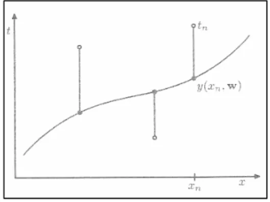
(2)

We simply note that it is a nonnegative quantity that would be zero if and only if the function y(x,w) were to pass exactly through each training data point. The geometrical interpretation of the sum-of-squares error function is illustrated in Figure 1.

Figure 1 The error function

We can solve the curve fitting problem by choosing the value w for which E(w) is as small as possible. The main problem is how we choose the order M of the polynom and as we shall see this will turn out to the problem of model comparison or model selection. In Figure 2, we show four examples fitting polynomials having orders M = 0, 1, 3, and 9 to the data set, which sample getting from a sinus function with noise.

Figure 2

Plots of polynomials having various orders M

The problems of the curve fitting and interpolation are that we do not understand the meaning of the parameters. In our approach we drop the traditional concept.

We define effects as a basic units, which have meaning. In Section 2 we define the basic units of the effects and we show how to create effect. In Section 3 we define how to compose and decompose functions. At the end we present some recent results.

2 Operations

In this section we present how to compose effect.

2.1 Sigmoid Function

A sigmoid function is a mathematical function that produces a sigmoid curve. We defined it by the following equation:

)

1

(

) 1

(

_{x a}

a

x e

_{− −}

= +

_λ

σ

λ (3)

where λ is the sharpness of the function and a is the offset. It is easy to see that

•

2

) 1 ( a =

a

σ

λ ,

•

σ

_a^−λ

( x ) = 1 − σ

_a^λ

( x )

.

2.2 Conjunction and Dombi Operator

To construct the effect we use fuzzy operators and sigmoid function. It is important to consider that the fuzzy operator and Dombi operator fits well. The operator is based on the solution of associativ function equation. The associative function equation is the following:

( ( ) ( ) )

) ,

( x y f

¹

f x f y

c =

⁻

+

(4)

This function c:

[ ] [ ] [ ]

0,1× 0,1 → 0,1, which is coninuous and satisfied the following properties:

• Commutativity:

c ( a , b ) = c ( b , a )

• Monotonicity:

c ( a , b ) ≤ c ( c , d )

, if

a ≤ c

and b≤d

• Associativity:

c ( a , c ( b , c )) = c ( c ( a , b ), c )

• 1 is an identity element:

c ( a , 1 ) = a

We get the Dombi operator by choosing:

x x x f

x x

f = −

⁻

= +

1 ) 1 ( 1 ,

)

(

¹ (5)

If we use the generator function in the conjunction case we get the following operator:

y y x

y x x

c = + − + −

1 1 1

) 1 ,

(

(6)

We can extend this with power and weight:

λ λ λ

λ 1

1 1 1

) 1 , , , (

⎟⎟

⎠

⎞

⎜⎜

⎝

⎛

⎟⎟⎠

⎜⎜ ⎞

⎝ + ⎛ −

⎟⎠

⎜ ⎞

⎝ + ⎛ −

=

y v y x

u x v

u y x

c , u+v=1 (7)

In this case we lose the associativity property.

2.3 Aggregation

Aggregation is not a logical operator. The form of an aggregation operator is:

∏

=

−

− + −

= _n

i i

i n

x x x

x a

0 0 0

1 1

1 1 1

) 1 ,..

(

υ υ υ

υ

^{, (8)}

where ν is the neutral value and ν0 is the threshold value of the corresponding negation.

The aggregation operator satisfies the following properties:

• Defined on [0,1] interval:

∪ [ ] ^{0 , 1}

ⁿ

^→ [ ] ^{0 , 1}

^,

• Identity when unary:

a ( x ) = x

, if

2 1

0

= υ =

υ

,

• Boundary Conditions:

a ( 0 ,..., 0 ) = 0

and

a ( 1 ,..., 1 ) = 1

,

• Non decreasing:

a ( x

₁

,..., x

_n

) ≤ a ( y

₁

,..., y

_n

)

if

) ,..., ( ) ,...,

( x

₁

x

_n

≤ y

₁

y

_n .

• Selfduality:

a ( n ( x ), n ( y )) = n ( a ( x , y ))

3 Function Composition and Decomposition

We deal a function, which is defined on [0,1] interval. In order to working in [0,1]

interval we have to transform the real function to [0,1]. This can be done by using a linear function or using the Sigmoid function.

To achieve our objective we will use Sigmoid function, Dombi operator, Conjunction operator and Aggregation operator. First we need natural effect, so we use two Sigmoid (3) function, and the conjunction operator (5):

) ( ) ( ,

,^{1 2} _{1 2}

1 ) 1

(

_{x a x b}

b

a

x e e

eff

_{− − − −}

+

= +

_{λ λ}

λ

λ (9)

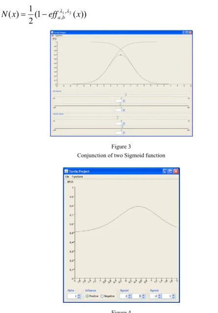
In Figure 3 you can see this effect. We define positive effect, which means that this effect will increase the function value and we define negative effect, which is the opposite of the positive effect (ie. decrease the function value). We define the positve effect on [1/2,1] and negative effect on [0,1/2]. The neutral value is 1/2.

To achieve this we need the proper transformation of (9):

)) ( 1

2 ( ) 1

( x eff

_,^{1, 2}

x

P = +

_a^λ_b^λ (10)

)) ( 1

2 ( ) 1

( x eff

_,^{1, 2}

x

N = −

_a^λ_b^λ (11)

Figure 3

Conjunction of two Sigmoid function

Figure 4 Positive Effect

In Figure 4 you can see that this function has four parameters. These parameters have semantic meanings: a is the starting point of the effect, b is the end point of the effect and lambdas are the sharpness of the effect.

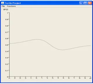
The last step of function creations is to aggregate these effects as you can see in Figure 5.

Figure 5 Aggregation of effects

In function decomposition we know the values. Our task is to divide real values into effects. It is an optimization problem. The critical point of the optimization is the initial values of the effects. If we define good initial points we have a high chance to find the global optimum.

In our case it is not impossible. We can define the number of the effect and each effect we can determine the following properties:

• Start/end point of the effect

• Sharpness of the effect.

4 Result

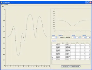
We create a Java program to create and analyze our approach. In our system we can create any arbitrary funcion as you can see in Figure 6.

Figure 6 Our Java system

The global optimization is under development in our Java system, but we tried in Matlab and the solution calculates very fast the parameters and the error of the result is acceptable.

Conclusions

In this paper we develop a new tool, that is useful for interpolation. Our approach has good properties. Our model is based on fuzzy logic. We create effects and aggregate them. Our method is also capable to decompose a function. We are working on an global optimization algorithm that is working in our System.

References

[1] Dombi J.: A General Class of Fuzzy Operators, the De Morgan Class of Fuzzy Operators and Fuzziness Measures Induced by Fuzzy Operators, Fuzzy Sets and Systems, Vol. 8, 1982, pp. 149-163

[2] Dombi J.: Basic Concept for a Theory of Evaluation: the Aggregation Operator, Europian Journal of Operations Research, Vol. 10, 1982, pp.

282-293

[3] Detyniecki M.: Fundamentals on Aggregation Operators, asturias, 2001