redevelopment – Advantages and disadvantages of quick-look geologic modeling

(1)

redevelopment – Advantages and disadvantages of quick-look geologic modeling

ISTV AN NEMES

^p

, SZILVIA SZIL AGYI SEB OK and } ISTV AN CSAT O

MOL Group, Oktober huszonharmadika u. 18., H-1117, Budapest, Hungary

Received: June 06, 2020 • Accepted: December 14, 2020 Published online: March 26, 2021

ABSTRACT

Due to the global oil price crisis in 2014, one of the MOL’s preventive/reactive measures was to identify geologically or commercially risky elements within their portfolio. This involved reevaluation of all geologic data from Field A in the Volga-Urals Basin. In re-evaluating Field A, several unexpected challenges, problems and pitfalls were faced by the interdisciplinary team performing the task of building a new database, quality checking, and interpreting data dating back to 1947. To overcome these challenges related to this matureﬁeld, new approaches andﬁt-for-purpose methods were required in order to achieve the overall goal of obtaining a reliable estimation of remaining hydrocarbon potential.

In thefirst phase afirst-pass 3D geologic model was constructed, along with wrangling, cleaning and interpreting 70 years of subsurface data. This paper focuses on the main challenges involved in evaluating or reevaluating reservoir aspects of a maturefield.

The primary challenges were related to the estimation of remaining in-place hydrocarbon volumes, the optimization of infill well placement, the identification of primary and secondary well targets, the identification of critical data gaps, and the planning of new data acquisitions. The hands-on experience gained during the development of the geologic model provided invaluable information for the next steps needed in the redevelopment of the field.

KEYWORDS

mature field, reservoir geology, reservoir modeling, field development, workflow

INTRODUCTION

By 2018 approximately 75–80% of the world’s total oil production was coming from mature ﬁelds. This, combined with the need to reduce unit costs due to a worldwide drop in oil prices (Fig. 1), put pressure on operators to reevaluate elements of their portfolios (O'Brian et al., 2016). Manyﬁelds had decades of production history, and a vast amount of data with a wide vintage and quality range, that makes redevelopment and optimal planning a challenging task. On the other hand, surface facilities were in place and there was an understanding of the subsurface geology. However, much of the available data needed to be upgraded or, in some cases, totally reinterpreted. The key to success was to have a multidisciplinary team working with a consistent, quality checked dataset so that no critical aspect was overlooked during reevaluation (Parshall, 2012).

Due to combined, interrelated reasons of slower than anticipated economic growth in China, Russia, India and Brazil, coupled with the upturn of unconventional exploitation in the US and Canada, crude oil prices dropped significantly since mid-2014 (Tarver, 2015;

Krauss, 2017; Depersio, 2019) (Fig. 1).

The abrupt oil-price drop in 2013–2014 (Fig. 1) triggered unprecedented cost reduction efforts by the oil industry. Cost-cutting actions were initiated, and portfolio optimization processes began. High-investment demand and/or high-risk projects ceased, and tens of

Central European Geology

64 (2021) 2, 74–90 DOI:

10.1556/24.2021.00003

ORIGINAL RESEARCH PAPER

pCorresponding author.

E-mail:isnemes@mol.hu

(2)

thousands of people were laid off (Bowler, 2015). Oil com- panies’ upstream sectors were compelled to adjust their strategies which included revisiting their mature assets. The redevelopment cost of mature elements of a portfolio is comparable to or even signiﬁcantly lower than new exploration costs. Moreover, redevelopment has lower risk than new exploration (Parshall, 2012; McComb & Towler, 2013).

Similar redevelopment efforts took place worldwide (O'Brian et al., 2016). A few examples are from Russia (Golovatskiy et al., 2015), India (Sarkar et al., 2015; Tiwari et al., 2015), Indonesia (Waskito et al., 2015), Malaysia (Ng et al., 2016), Australia (Mantopoulos et al., 2015), Egypt (El-Bagoury et al., 2017), China (Rajput et al., 2015), among many others.

At MOL Group (Hungarian Oil and Gas Public Limited Company), the existing portfolio was revised to minimize risk and maximize value. Similar approaches are described by Golovatskiy et al. (2015), Sarkar et al. (2015), Tiwari et al.

(2015), and Rajput et al. (2015). The goal was to transform the business to withstand abrupt market changes. In the case of MOL, the strategy illuminated the urgent need for a thorough reevaluation of Field A’s (Fig. 2) hydrocarbon volumes and further development potential. In order to re- estimate theﬁeld potential, a standardized, quality-checked, and comprehensive subsurface database was constructed.

This required that much of the existing data be reinterpreted.

The key disciplines involved in this multidisciplinary task were geophysics, petrophysics, fluid and core laboratory studies, sedimentology, geology, reservoir geology, reservoir engineering, drilling, completions, and well testing. Nowa- days no major projects are initiated without the integration of multiple disciplines (Baillie et al., 1996; Campobasso et al., 2005; Okuyiga et al., 2007; Galindo et al., 2012; Ringrose &

Bentley, 2015; Sarkar et al., 2015; Lukmanov & Ibrahim, 2018). Data governance and database maintenance were provided by the data management department (Akoum &

Hazzaa, 2019). The optimal solution to meet redevelopment goals is to build a 3D geologic model and, based on this model, a 3D history-matched dynamicﬂow model. Theﬂow model can serve as an effective tool for developmental planning and estimation of remaining potential (Papay, 2003; Ringrose & Bentley, 2015).

First, a low complexity, deterministic geologic model was built (Phase 1), and simultaneously preparations were made for a second (Phase 2), detailed and multi-realization geo- modeling aiming to more realistically reflect the actual behavior of the field and incorporating data and understanding not available at the time of the first model.

This paper aims to discuss the work conducted during the first modeling job, identify data gaps and bottlenecks as well as discuss plans that support the improvement of the understanding of the reservoirs.

The main goal of Phase 1 modeling was to make a quick, preliminary in-place volume calculation. The comparison of the results with historical data enabled a rough estimation of volume changes both in terms of in-place and remaining recoverable resources to be made. A partly hidden layer of the modeling job is its underlying psychological effect, such as in the case of verbal or written communication. It helps to structure thoughts and ideas, knowledge and information.

Practically, it separates dead-ends from viable options and highlights critical elements while depressing insignificant details. It had a vast effect on the next steps in terms of highlighting data and knowledge gaps, inconsistencies and contradictions.

The Phase 2 model will utilize a more complete input dataset, more sophisticated modeling methods and a full- cycle, automated workflow providing a tool applicable in daily operations, and function as a single source of subsurface data. Secondly, it will incorporate all the experiences gathered during the Phase 1 history-matching process.

Thirdly, it will incorporate all the relevant new data and information acquired during the time interval between the two models.

GEOLOGIC SETTING, TECTONICS AND STRATIGRAPHY

Field A is an onshore oil field, located in the central part of the Volga-Urals Basin, south of the South Tatar Arch (Fig. 2) and the Romashkinskoye oil ﬁeld. The ﬁeld is geographically situated in the southern part of the Russian Fig. 1.History of Brent oil prices since 2010. Brent prices peaked above $110/bbl (barrel) in late 2013, plummeted below $30/bbl in 2015 and eventually stabilized around $50/bbl (Campbell, 2017; Redden & Strickland, 2017). (Source of data:https://www.eia.gov/(18-04-2020))

(3)

Federation, 400 km north of Kazakhstan on the border of the Orenburg and Samara regions (Zozulya et al., 2016).

The Volga-Urals basin with its acreage of approx.

700,000 km² is the second most proliﬁc HC-region (hydrocarbon region) in the Russian Federation – after Western Siberia–spreading from the Urals geosyncline on the east, to the Volga river and Russian platform on the west and the Caspian basin to the south (Parfenov et al., 2008;

Meyerhoff, 1984).

The main structural features of the Volga-Urals Basin were formed by several tectonic stages, during which many arches and local uplifts (for instance the Volga-Ural anticline itself), depressions and grabens were formed (Fig. 2).

Despite later deformations, the basement surface bears the marks of most of the older tectonic movements except for

the younger sedimentary troughs and reef buildups (Peter- son & Clarke, 1983). The basement complex in the area consists of Precambrian crystalline rocks deepening toward the Precaspian Basin and the Ural Mountains to the east (Fig. 2).

Most Soviet authors agree that in the Volga-Urals region tectonic development played a major role in the accumula- tion and trapping of hydrocarbons. A detailed tectonic and structural scheme of the Volga-Ural anticline and region was given by Smirnov et al. (1958), Guseva et al. (1975), ONAKO (1997) and Kolchugin et al. (2014). As a result of the intensive drilling activity during the decades of exploration and production in the Volga-Ural Petroleum Prov- ince, the deep structural elements and tectonic features are relatively well known. Amongst them, the Sernovodsko- Fig. 2.Structural schematic map of the Pre-Paleozoic basement of the Volga-Urals Basin. The black rectangle indicates the approximate location of Field A (depth contours digitized afterPeterson and Clarke, 1983; IHS)

(4)

Abdulino graben to the south and the Kazansko-Kirov- South graben to the west surround the study area (Fig. 2).

The structures of the area are related to six distinct episodes of tectonic activity in the basin (Volga-Urals Basin report, IHS). The events resulted in Riphean-Vendian rift structures, Late Cambrian-Silurian passive margin structures due to the development of the Ural Ocean, Early Devonian compressive structures related to the Caledonian Orogeny, Middle Devonian-Mid Carboniferous rift structures, Late Carboniferous-Triassic Uralian compressive structures con- nected to the foreland basin formation of the Ural Mountain Belt, and Oligocene to recent compressive structures due to late reactivation of thrusts and faults.

Golov et al. (2000)divided the evolution into three main stages: a Middle Devonian extension, a passive margin subsidence in the Upper Devonian through the Permian, and a tectonic inversion in the Permo-Triassic, which was rejuvenated later in the Cenozoic Era. Carbonate deposition

increased markedly during the Famennian, when reef and organic carbonate deposits covered most of the Volga-Ural province (Fig. 3). The highly bituminous Domanik facies, which later served as source rock, continued to be deposited in troughs. The Domanik facies is thinner and less silty than that of the Frasnian.

The general emergence of the Russian Platform occurred following the deposition of Tournaisian reefal and other carbonate facies. A cyclic transgressive-regressive marine deposition took place following the Tournaisian, producing a thick interfingering nearshore deltaic/interdeltaic marine and continental-coastal clastic sequence. The clastic sequence had a major effect on the distribution of petroleum reservoir sediments and source rocks of the Volga-Ural Petroleum Province (Peterson & Clarke, 1983). Deposition of clastic sediments in Visean time completed theﬁlling of the troughs. The major source area for Visean clastics was the Baltic Shield to the northwest.

Fig. 3.Simpliﬁed lithological column and geologic stages of the Early Devonian-Permian in the AOI (area of interest) (modiﬁed afterHaq and Schutter, 2008 and Peterson and Clarke, 1983, IHS Markit)

(5)

Subaerial exposure of carbonates occurred at the end of the Tournaisian, as well as at the ends of the Serpukhovian and of the Bashkirian. These events induced karstification and formation of dissolution features in the limestone. The most wide-spread and significant karstification effect is present in the Serpukhovian Formation; there is a slight effect in the Bashkirian Formation and a negligible one in the Tournaisian.

SEDIMENTARY SEQUENCES OF THE AREA AND HYDROCARBON RESERVOIRS OF THE FIELD

Four major Paleozoic sedimentary sequences are usually re- ported in literature from the Volga-Urals Basin. These are the Eifelian-Tournaisian, Visean-Bashkirian, Moscovian-Artin- skian, and uppermost Kungurian. Each of them may be further subdivided to shorter-term sequences that correspond to relative sea level changes (Peterson and Clarke, 1983). In Field A the primary hydrocarbon-bearing reservoirs are of Carboniferous age: the Tournaisian (V1), Bobrikovian (Bb), Serpukhovian (C1s), and Bashkirian (A4) formations (Fig. 3).

A moderately dynamic depositional environment is presumed for theTournaisian Formation (V1), according to shape and size of peloids, representing a shallow water shelf with normal benthic fauna. Lithologically the formation is comprised mainly of limestone, characterized by vuggy porosity.

In Field A the interpreted depositional environment for the Lower Visean Bobrikovsky Formation (Bb) is a nearshore/coastal one which was located in the broad shallow shelf of the Volga-Urals Basin. Barrier islands were formed in enclosed lagoons and estuaries. Tidal deltas, including flood tidal and ebb tidal deltas with tidal channels and bayhead delta sediments, were deposited in and in front of the lagoonal series. The pore volume is dominated by matrix porosity that shows high heterogeneity among the different facies. Sandstone, siltstone and shale layers make up the formation. The high level of heterogeneity has a significant effect on the productivity of wells that produce from this formation. The daily total fluid production ranges from 1-2 m³to 60–80 m³. The base of the formation is marked by theMalinovsuperhorizon which starts with dark grey, thin bedded shale and claystone, with pyrite crystals that were deposited under anoxic conditions in relatively deep-water environments (Ulmishek, 1988).

The Serpukhovian (C1s) Formation consists of marine limestone with a signiﬁcant level of diagenetic dolomitiza- tion. Brief emergence and erosion occurred at the end of the Serpukhovian when karstiﬁcation affected the rocks, resulting in vuggy pores and paleokarstic features.

Fossil analysis from rocks of the Bashkirian Formation (A4)suggests a shallow marine, well-circulated environment.

Based on the shape and size of peloids, a moderately agitated open marine and inner ramp environment is presumed. The most characteristic pore type is vuggy porosity, supple- mented by intraskeletal pores. The average pore size is larger than in the Tournaisian Formation. Lithologically the

formation is mainly limestone with a subordinate amount of dolomite, with a high degree of heterogeneity due to diagenetic processes.

MATERIALS AND METHODS

Brief history of the field

A valued and interesting resume of the oil and gas industry’s exploration of the Volga-Ural Petroleum Province’s two historical centers’ – Tatarstan and Bashkortostan – was presented byKontorovic et al. (2016). The early exploration activities and geologic surveys had been conducted in the second half of the 18th century thanks to expeditions of academic scientists. Theﬁrst occasional oil inﬂow was noted in 1929 during exploration for potash near the village of Verkhne-Chusovskie Gorodki (Kontorovich & Livshits 2017).

The neighboring Orenburg (and Samara) oil regions, where Field A is situated, are some of the oldest in the Russian Federation. The first discoveries were made in the 1930s. The huge and easy-to-recover reserves are in a mature or nearly depleted stage, and new cutting-edge technologies are needed to continue exploitation and to extend field lifetime (Shakirov et al., 2015).

Field A was discovered in 1947 and production began in 1949; consequently, the acquired data reflects the techniques and methods of seven decades. The result is that data varies highly both in quantity and quality, fundamentally pre- defining the extractable amount of information. The first wells show the initial reservoir conditions and parameters that are essential to constructing a reservoir model. While later wells have higher-resolution and more reliable data, they can show a non-initial state of the parameters (e.g., saturation profile). An intensive drilling campaign started after 2007, when MOL obtained 100% equity in the field.

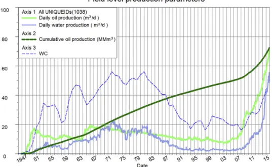
Due to the market environment and reservoir behavior the field development strategy has been to employ mainly infill drilling with a regular drilling pattern of 4–500 m between wells. From 2007 to 2016 40–70 wells have been drilled per year. These wells provide a significant amount of data and have ramped up the daily production (Fig. 4).

The actual recovery factor at the end of 2015 was approximately 8–12% (depending on STOIIP – stock-tank oil initially in place). The relatively low recovery factor suggests that a detailed investigation may identify new opportunities and adjustments to optimize production and, hence, maximize profits (Papay, 2003).

Applied methods

At the start of Phase 1 geologic modeling, numerous types of input data had not been completely finalized. Therefore, it was necessary to track in detail what those data are, or which information gaps were being revealed that need to be miti- gated before Phase 2 modeling begins. This approach of modeling was triggered by business needs, but always underlining that the outcomes of Phase 1 cannot be handled

(6)

as final results. The vintage of the Phase 1 model is 01-01- 2016; no later data were incorporated during the modeling process, in order to achieve a consistent state that can be regularly updated once prepared.

Hydrocarbons in Field A are produced from four formations, three carbonate (V1, C1s, A4) and one clastic (Bb).

All four formations were incorporated in the 3D geologic model shown inFig. 5. The schematic section indicates true vertical depth in meters below sea level (500–1,000 m TVDSS) for the four formations.

The A4 and C1s formations are separated from the Bb and V1 formations by approximately 300 m of impermeable rock (Fig. 5). However, hydrodynamic communication of the stacked pairs is probable even though there is a shale

layer partly separating them (Flow-barrier between A4 and C1s and the Malinov Shale between Bb and V1) (Fig. 5).

A repeatable, iterative modeling workflow was outlined with Roxar’s RMS 2013.1 software covering the key steps of the modeling. The workﬂow followed a common suite of procedures, beginning with fault and horizon modeling, structural modeling, building a 3D grid, populating the 3D grid with facies and petrophysical properties and calculating hydrocarbon in place volumes (Fig. 6) (Adelu et al., 2019;

Kaleta et al., 2012; Shirazi et al., 2010; Spagnuolo et al., 2018).

It should be noted that the geologic model presented herein was replicated in Schlumberger Petrel 2015.5 because of business requirements. There were marginal differences in Fig. 4.The accelerated drilling campaign initiated in 2007 had a signiﬁcant impact on daily production (data is aggregated for 1,038 wells completed between 1947 and 2016). The left axis shows water cut (WC–ratio of oil and total liquid production in volume percentage). The reminder of the qualitative data falls under a non-disclosure agreement

Fig. 5.Schematic N–S cross-section across Field A showing the stratigraphic framework, as well as the impermeable shale layers and reference case OWCs (oil-water contact) (Z-scale510.00). The vertical lines indicate projected well trajectories. A4, C1s, Bb, and V1 represent the Bashkirian, Serpukhovian, Bobrikovian, and Tournaisian Formations, respectively. A4 and C1s are partially separated by an impermeable bafﬂe zone, called Flowbarrier. Bb and V1 formations are separated by the Malinov Shale. The dashed blue lines represent the initial oil-water contact for each formation

(7)

the results of the two programs, mainly resulting from sto- chastic deviations. All the differences, however, were within the standard deviation for any given parameter defined in each software.

The corresponding types of input data at each step of the applied workflow are shown inFig. 6. It should be noted that the input data listed are only the main, primary data directly used for Phase 1 geologic model of Field A.

RESULTS

Structural and grid modeling

At the vintage of the geologic model (01.01.2016) the actual stock of wells consisted of 459 wells, of which 349 had measured (and digitized) trajectory data, 46 were available only in paper format and 64 had no deviation survey. The latter two groups were handled as vertical wells with their data considered highly uncertain. Most of the wells are vertical or slightly deviated, but during a pilot project 13

horizontal wells were also drilled. These wells required special attention during the modeling process in order to avoid anomalies in structure or in property modeling. To have an up-to-date set of well attributes, a detailed well register was created (Fig. 7).

The geologic model was constructed following the workflow diagram shown inFig. 6. This is a general work- ﬂow applied in numerous modeling exercises in simple (Adelu et al., 2019) or in more complex forms (Galindo et al., 2012; Kaleta et al., 2012; Shirazi et al., 2010; Spagnuolo et al., 2018).

The main input parameters for the structural model were the interpreted seismic horizons (Fig. 8 and Fig. 12) (stratigraphic tops and bottoms) and fault sticks. The subseismic intralayers were mapped using the well picks. Well picks (stratigraphic) were checked and ﬁltered prior to use for adjusting the seismic interpretation. The well data were handled as hard data (Ebong et al., 2019) (Table 1). The structural modeling was performed in the depth domain.

The seismic interpretation was performed in the time domain and converted to depth (Fig. 12).

Fig. 6.Schematic overview of a general workflow applied in 3D geologic modeling. The main inputs at the corresponding steps (on the left) are those used in the current modeling phase of Field A (Note that the 3D geologic model is an input to the 3D dynamic model, and not its result; hence not an end of the workflow). On the right the colors indicate the main stages of geologic modeling, and the boxes represent the individual steps. Input data and corresponding modeling steps are linked by arrows showing the direction of dataflow

(8)

Well-pick filtering was necessary due to the unreliability of some input data. In some cases, the well trajectory, the well log’s depth or the interpretation was dubious. The mapping increment was 20320 m due to the high density of wells (average well spacing is approximately 4–500 m).

The mapping algorithm used was Global B-spline (Roxar, 2012). The isochore picks were calculated based on the horizon picks and were later used during structural modeling in order to control the pinch-outs of the Flow- barrier and the Malinov Shale.

The oil–water contacts (OWC) were identified based on formation testing data; however, in several cases contradictions occurred for various reasons, e.g., measurement quality, cement bond quality, log quality and/or influence of injection or production in the vicinity. Identification of free water level (FWL) was attempted, but due to numerous contradicting interpretations, the empirical OWCs were used for gross rock volume (GRV) calculations, though leaving the question of hydrodynamic connectivity unset- tled.

The structural modeling followed three main successive steps: fault modeling, and a nested two-step horizon modeling that resulted in a structural model as the main input used for 3D gridding (Fig. 6).

The first step in constructing the model included only the main horizons (Fig. 8), while the second step was nested into the outcome of the ﬁrst step, adding the thin layers of Flowbarrier and Malinov Shale. One major and several

smaller faults were identiﬁed on seismic records; these were incorporated in the model. The major strike-slip fault in the east is a bounding fault, it provides the closure to the east (Fig. 8). It should be noted that later investigations revealed minor or no role of faults on ﬂow behavior; hence to simplify the grid, the faults were removed from the model.

Because of the identified heterogeneity of individual formations, the vertical resolution of the 3D grid was set to 1 m for the carbonate reservoirs, and 0.4 m for the clastic reservoir. In all cases corner-point gridding was used without rotation, but the 3D grid was clipped with a pre- defined polygon. The horizontal resolution was set to 50 m for the geologic grid; later it was upscaled for flow modeling (Table 2). Gridding was set up taking into consideration the unconformity at the top of Tournaisian and Serpukhovian formations, while stair-stepped fault handling was applied for dynamic modeling. In order to honor the high-conﬁ- dence well picks the 3D grid was also adjusted to the picks prior to property modeling (Table 1).

Upscaling of well logs

The aim of well log data upscaling – or also known as blocking – is to synchronize the vertical resolution of the petrophysical logs with the 3D grid (Zakrevsky, 2011). As computational performance increases exponentially according to Moore’s law (Moore, 1965), the magnitude of upscaling can be decreased. In some cases, no upscaling is Fig. 7.A snapshot of the well register showing several well attributes such as core, status, artiﬁcial lift system (e.g., SRP–sucker rod pump), spud date from Roxar RMS's Well Administration Tab, etc. Colors are automatically attributed to the corresponding attribute's values

(9)

necessary, i.e., the resolution of the 3D model is equivalent to those of the well logs (it must be noted that the log data intrinsically represent average values for the resolution limit of the given tool type).

Interconnected porosity, initial water saturation and reservoir flag parameters were upscaled. The cutoffs were identified for each formation individually, based on integrated petrophysical interpretation of logs, core and well test data in the case of V1, C1s, and A4 porosity cut, while in the case of Bb porosity and shale cut was applied.

Discrete type-reservoir flag was upscaled using most of the algorithm, while in the case of continuous parameters

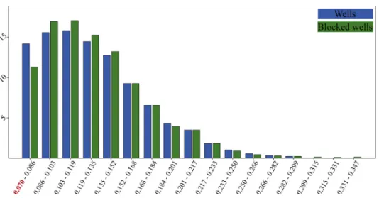
arithmetic averaging was applied biased to reservoir flag (The reservoir flag consists of discrete 1 and 0, i.e., reservoir and non-reservoir values). The shift-and-scale method was used in order to match the grid zones pre- cisely with the zone log(Roxar, 2012). Histograms were used to validate the upscaled results as shown in Fig. 9 (El-Bagoury et al., 2017).

Rock-type modeling

New, standardized and integrated petrophysical interpretation was conducted in the case of 318 wells, including quality Fig. 8.Structural top map of the C1s Formation with well picks (green discs) used for anchoring the depth horizon, indicating 3D seismic coverage (white) and license boundary polygon (blue). The eastern N–S strike-slip fault is the eastern bounding fault of theﬁeld (along the license boundary). In other directions structural deepening bounds the HC accumulations (dark green line indicates the external OWC polygon)

(10)

flag logs in order to be able to filter unreliable data during modeling.

A sequential indicator simulation (SIS) (Ringrose and Bentley, 2015) technique (pixel-based) was used for modeling of rock types (reservoir and non-reservoir) in the case of all formations. SIS is useful where the reservoir elements do not have discrete geometries, either because they have irregular shapes or variable sizes; that is the case in the carbonate reservoirs of Field A. SIS also gives good models for reservoirs with high well density (Ringrose & Bentley, 2015). In the case of Bb, reservoir facies analysis was in progress during the modeling; hence SIS was applied using no direct trend maps.

Vertical Proportion Curves (VPCs) were introduced as vertical trends; and in the case of Flowbarrier and Malinov

Shale, the reservoir flag was manually set to 0, meaning non- reservoir (Fig. 10). The output 3D parameter can be directly applied as a net-to-gross (NtG) multiplier (see Eq. (3)), or as a discrete filter for volumetric calculations. The NtG parameter defines the ratio of the thickness of an interval capable of providing fluid flow to the total thickness.

A common practice is to calculate the value by applying cut-off values, which are predeﬁned criteria (porosity, shale content, permeability) to distinguish reservoir and non- reservoir rocks (A logical expression to illustrate application of cut-offs: IF (Porosity > 11% AND Shale < 40%), THEN NtG51, ELSE NtG5 0 ENDIF).

Petrophysical modeling

Petrophysical modeling of interconnected porosity (Fig. 12) and water saturation was performed biased to previously modeled reservoir ﬂag parameter. The modeling was conditioned to blocked well data, and the statistical range of parameters set to honor the input data.

Interconnected porosity was modeled separately for each formation and rock type using the basic function of geo- statistics, variograms (Fig. 11). This method is commonly used to assess the spatial autocorrelation (continuity or variability) of a reservoir variable (Roxar, 2012; Ringrose and Bentley, 2015). Log-derived water saturation was modeled co-simulating with porosity. During the analysis empirical and theoretical semivariograms wereﬁtted to approximately 10,000 data points from 350 wells with estimation settings updated formation by formation.

Since all the wells with interpreted saturation curves were used, this resulted in a probably slightly conservative estimation of hydrocarbon pore volume (HCPV) due to the (non)-representativity of new wells regarding initial saturation profile. A study previously conducted has shown the advantage of Thomeer-curve fitting to MICP (Mercury injection capillary pressure) drainage curves (Nemes, 2016).

An attempt was made to use similar methods in the case of Field A, but the initial results were contradictory, and the scarcity of input data reduced accuracy compared to log- derived water saturation proﬁles.

Water saturation cut-off was applied to the 3D grid, resulting in a pay-flag discrete parameter, used for net pore volume (NPV) calculation during the next step.

Permeability was calculated based on the porosity applying porosity-permeability regression equations identified on core measurements (see Eq. (1) for Bobrikovsky Forma- tion and Eq. (2) for Tournaisian Formation as examples):

log PermeabilityðmDÞ ¼ ðlog Porosityð%Þ 1:31Þ=0:1815 (1) log PermeabilityðmDÞ ¼ ðlog Porosityð%Þ 1:26Þ=0:0962 (2)

Volume calculation

Having modeled all the input variables for in-place volume calculations and deriving an initial formation volume factor Table 1.The table shows the number of well tops (i.e., well picks)

used for structural modeling, normalized by license area (≈largest reservoir area). Unreliable data points were removed from the dataset for further investigation beyond the scope of modeling

Horizon

Number of well picks (post-filter)

Average number of well picks per unit area

(1/km²)

A4 Top 350 5.3

Flowbarrier Top

325 4.9

C1s Top 319 4.9

C1s Bottom 279 4.2

Bb Top 314 4.8

Malinov Top

311 4.7

V1 Top 312 4.7

V1 Bottom 179 2.7

Table 2.Main parameters of the 3D grid for geologic modeling. All four reservoir zones were included in one 3D grid, non-reservoir

zones represented by one cell/layer Grid layout

Format Corner point

Rotation angle 08

Total number of cells 30,801,429

Number of deﬁned cells 14,264,165

Number of undeﬁned cells 16,537,264

Number of columns 223

Number of rows 447

Number of layers 309

Number of simbox columns 220

Number of simbox rows 446

Number of simbox layers 309

Number of zones 7

Zone 1 Layers 1–70 A4

Zone 2 Layers 71–71 FlowBarrier

Zone 3 Layers 72–163 C1s

Zone 4 Layers 164–164 Non-permeable interlayer

Zone 5 Layers 165–228 Bb

Zone 6 Layers 229–229 Malinov

Zone 7 Layers 230–309 V1

(11)

(Boi) (Danesh, 1998) for all the reservoirs, STOIIP estimation was possible. The widely applied equation for calculating stock-tank oil initially in place is shown in Eq. 3.

STOIIP¼GRV*NtG*4*ð1SwiÞ

Boi (3)

whereSTOIIPis stock-tank oil initially in-place (m³),GRVis gross rock volume (m³),NtGis net-to-gross ratio (%), 4is

interconnected porosity (%), Swi is initial water saturation (%), and Boi is formation volume factor at initial reservoir conditions (m³/sm³). The calculations were made using different polygon sets according to administrative and leg- islative requirements. The key result was that, due to a combination of area and net thickness parameter changes, compared to the latest study the STOIIP showed a total increase of 20–40%.

Fig. 9.Example (porosity of C1s Formation in the reservoir intervals) for cross-validation of pre- vs. post-upscale (blue and green respectively) data probability distribution (histogram). Note that the minimum value is 0.070, reﬂecting the porosity cut-off for reservoir vs.

non-reservoir. Number of observations: approximately 400,000 (based on∼320 wells' data)

Fig. 10.Vertical Proportion Curve (VPC) represents a given discrete variable's vertical distribution and serves as a vertical trend in modeling. The vertical axis represents the 3D model's simbox layers, while the horizontal axis shows the proportions. The color red indicates the non-reservoir, green the reservoir rock type in the Bobrikovsky Formation. Higher reservoir ratios (sandy parts) can be identiﬁed near the bottom and top of the formation. These sandy intervals are separated by a thick, shaly interval

(12)

DISCUSSION

The main goal of this section is to summarize the key findings that were obtained and/or implemented during Phase 2.

Geologic and dynamic modeling techniques (incorporating surface facilities also) have been widely used in the

petroleum industry for decades (Adelu et al., 2019; Dehghani et al., 2006; Gonzalez et al., 2008; Lurprommas et al., 2016;

Mantopoulos et al., 2015; Martino et al., 2012; Ringrose and Bentley, 2015; Sarkar et al., 2015; Spagnuolo et al., 2018;

Waskito et al., 2015). It should be noted that the use of new, data-driven methods is spreading in several industries, including the energy sector. An overview of these methods is Fig. 11.Illustration of 3D porosity variograms for the Bobrikovsky Formation applied in the petrophysical workﬂow (directions are with respect to azimuth; lag distances' unit is meters). During the modeling workﬂow approximately 100 variograms were applied (as per formation, rock type and parameter). Panel A.: parallel to azimuth direction, general exponential type, range is 725 m. Panel B.: normal to azimuth direction, general exponential type, range is 500 m. Panel C.: vertical direction, general exponential type, range is 3.5 m

(13)

given by Balaji et al. (2018). The re-modeling of Field A included the novel approach of splitting the modeling job into two phases in order to provide room for inevitable updates related to gaps being revealed during execution of the task.

Numerically the key results were the volumetrics (and the significant increase in STOIIP), and the reference case 3D geologic model with spatially distributed reservoir parameters, which could be used to start the dynamic modeling. The geologic model constructed during Phase 1 had a significant impact on the planning of new wells, both in numbers, placing, target interval, field development strategy and data acquisition program.

During Phase 1, gaps and bottlenecks were revealed that could have an impact on field development. Hence, these triggered action plans and a detailed to-do list for the Phase 2 modeling and the data acquisition prior to it.

Also, according to various authors worldwide, one of the key challenges related to mature fields is data availability, reliability and relevancy (Parshall, 2012), as case studies from Kazakhstan (Elliott et al., 1998; Bigoni et al., 2010), Russia (Cimic, 2006), Venezuela (Agbon et al., 2003), Indonesia (Handayani & Simamora, 2012), or India (Tiwari et al., 2015) show. Similar challenges were also identiﬁed in the case of Field A during Phase 1.

Thesoftwareto construct the geologic model apparently underwent changes in the time between the two phases. As mentioned earlier, the Phase 1 model, built in Roxar Irap RMS 2013.1, was later on rebuilt using Schlumberger’s Petrel

2015.5 as a result of customer requirements. The Phase 2 geologic model was initially constructed using Schlumberg- er’s Petrel software package for the same reason.

The dataset available at the time of closing of Phase 1 was not thefinal one used. Well trajectories, measured and interpreted log sets, core data, finalized completion and production logs, some historical reports and fine-tuned seismic interpretation were also missing. All the data integration, standardizing and quality checking to a common, single-source-of-truth database was initiated during Phase 1 modeling. The fit-for-purpose solution was to use a Petrel reference model, into which all the input and interpreted data was incorporated. These data can be seamlessly loaded into working projects at different locations, different experts using Reference Project Tool, thereby avoiding major con- versions of data and possible loss of information or data corruption. The same tool provides the opportunity to strictly fix the coordinate system, the templates, the nomenclature and unit system applied in order to decrease the chance of inconsistencies occurring among the same data records in different projects. A similar problem is outlined by Cimic (2006) related to mature Russian assets that are planned to be redeveloped and optimized.

In thestructural modelingseveral outlier datapoints had to be removed from the horizon adjustment procedure due to anomalous depth values compared to offset wells. The root cause of these anomalies had to be investigated one by one since they can have an effect on the spatial distribution of properties, or on completion data and production allo- cation. A subset of wells (∼30 wells) had a high impact on the modeling of the Bobrikovian Formation. This is important since these wells provided approximately 50% of historical production from the formation. These wells were all drilled in the 1950s and 1960s, thus having limited trajectory data and a very limited petrophysical log suite (SP, GR and/or RES) (Cimic, 2006). Also, the possibility of subzonation of the main horizons needed to be revisited in order to provide a higher degree of control on property modeling in later steps.

Inrock type (and petrophysical modeling)for the Bobri- kovian Formation (Bb), a need for trend maps became evident in order to be able to spatially distribute and frame the high degree of horizontal heterogeneity. In the case of the Serpukhovian Formation (C1s), the effect of paleokarstic features was not considered in the Phase 1 model, neither in terms of volumes nor inflow behavior. Modeling of paleokarstic features was performed by several experts, but still remains a challenge in order to establish a realistic model (Chung et al., 2011; Lurprommas et al., 2016; Shen et al., 2019). The subzonation of the Tournaisian Formation (V1) also played a significant role in property models, namely that the lower part of the formation shows lower permeability compared to the upper zone. This difference has a critical effect on the saturation profile, productivity and water encroachment. The permeability model was planned to have porosity-permeability regression curves updated by incorporating new results and through subzonation.

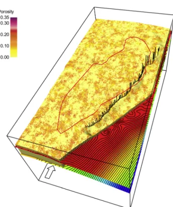
Fig. 12.Snapshot of the 3D output (porosity cube). The red polygon depicts the license boundary. The black sticks show the eastern bounding fault's skeleton that was an input for structural modeling along with the seismic horizons contoured in theﬁgure

(14)

A framework needed to be outlined, so that the model can be updated on a regular (biweekly) basis in a standardized, automatable manner, as new data (new wells, adjusted interpretations) became available. In order to structure these updates and save time a full cycle workflow will be defined from loading the data to the geomodel to updating of the volumetric calculations. Advantages of this workflow will be detailed in a succeeding publication.

Similar work was done byKumar et al. in 2017, but with a wider scope.

Acquisition of newwell log setswere proposed for some of the new wells, with the intention of mitigating part of the revealed information gaps and shrink the uncertainty of input parameters. These proposed logs are as follows: (1) Acoustic density logs in the shallow sections of wells to update the seismic velocity model, which lacks information of the upper 500 m of the depth range. (2) Image logs (FMI/CBIL/STAR) in order to have an alternative to short well tests to investigate the possible role of natural fractures on flow behavior. (3) Nuclear magnetic resonance logs (NMR) in order to investigate the in-site moveable and residual fluid saturation and permeability. (4) LithoScanner logs to increase the understanding of mineral composition, with emphasis on anhydrite content which plays a key role in porosity uncertainty. (5) Spectralog to differentiate uranium from clay minerals (Simultaneously the number of tools run as conventional logging set was rationalized; excess measurements were removed, e.g., induction log.) Additional core and fluid measurements were requested tofill-in data gaps mainly in permeability measurements, and oil properties.

Detailed geologic investigations were initiated based on the clues identified during Phase 1: Bobrikovsky facies analysis, old Bobrikovsky wells’ petrophysical investigation, Serpukhovian paleokarst mapping, hardcopy data digitali- zation (trajectory, production), and numerous minor adjustments (e.g., well name contradictions, wellhead elevation, log set anomalies).

CONCLUSION

The main result of the Phase 1 modeling exercise was that 70 years of data gathering and investigation started to become a structured set of understanding, where the focus points were revealed. Importantly, based on the results an action plan could be outlined to decrease the uncertainty related to the understanding of the field’s behavior and remaining hydrocarbon potential.

A main lesson learned is that a first-pass, non-sophisticated, coarse model is already capable of delivering a series of insights that can be directly applied in the daily operations of a field, and can deliver significant support in understanding the approximate remaining potential and development opportunities for an oil field. Also, a more sophisticated and up-to-date tool is needed to fully plan and realize these opportunities and estimate the associated risks and uncertainties.

It takes a huge effort to map the size of the task in the case of a project that aims to establish a general understanding of a field which, although discovered in 1947, still is not in a mature phase in terms of actual primary recovery factor, and thus having a huge remaining potential. In other words, by revitalizing this field the extracted value can be increased beyond original expectations (Parshall, 2012). The opportunity for further investigations and increased exploitation efforts was provided by a positive change in oil initially in place, naturally not being identical to an instant increase of value, but nevertheless a signiﬁcant milestone.

The preparatory work, the multidisciplinary interpretation and modeling all revealed new information, or outdated old, erroneous“beliefs”, something that is equally important and crucial on the road to transparency. As the quote credited to Mark Twain says:“It ain't what you don't know that gets you into trouble. It’s what you know for sure that just ain't so.”

The outlined methodology can be a useful tool for industry professionals dealing with mature fields with a wide variety and reliability of data, facing significant data gaps (e.g., Central and Eastern-European hydrocarbon reservoirs). It is a quick and effective workflow to build a basic understanding and quantification of the field behavior and potential, focusing on the crucial aspects and identifying critical momentums.

Although the updating of the Phase 1 model was crucial and inevitable for several reasons: new gathered data, reinterpreted data, old data became available, mitigation of non-suitable modeling steps, incorporation of experiences gathered during first-pass history-matching process, establish a fully integrated workflow and mainly to gain a better tool for a 3D representation of the subsurface characteristics of Field A.

ACKNOWLEDGMENTS

We would like to express our appreciation and greatest gratitude to every former and actual colleague, who worked or is still working on the project, be it in Russia, in Hungary, in Spain, in Turkey or anywhere else in the world. It was an honor to work with them, to learn from them and to add our efforts to this exciting, adventurous, challenging, but also professionally and personally highly rewarding task.

Table 3.List of acronyms and units

Acronym Description Unit (if any)

AOI Area of interest –

A4 Bashkirian Formation –

Bb Bobrikovian Formation –

Boi formation volume factor m³/sm³

C1s Serpukhovian Formation –

CAPEX capital expenditure million USD

CBIL circumferential borehole imaging log –

FMI formation micro-imager –

(continued)

(15)

REFERENCES

Adelu, A.O., Aderemi, A.A., Akanji, A.O., Sanuade,O.A., Kaka, S.I., Afolabi, O., Olugbemiga, S., and Oke, R. (2019). Application of 3D static modeling for optimal reservoir characterization.

Journal of African Earth Sciences, 152: pp. 184–196.

Agbon, I.S., Aldana, G.J., Araque, J.C., Mendoza, A.A., and Ram- irez, M.E. (2003). Resolving historical-data uncertainties for redevelopment of matureﬁelds.Journal of Petroleum Technol- ogy, 56(1): 38–79, https://onepetro.org/journal-paper/SPE- 0104-0038-JPT.

Akoum, M. and Hazzaa, H.B. (2019). A data governance framework–the foundation for data management excellence. SPE, 198593.

Baillie, J., Coombes, T., and Rae, S. (1996). Dunbar reservoir model, a multidisciplinary approach to update brent reservoir description and modelling. https://onepetro.org/conference- paper/SPE-35528-MS.

Balaji, K., Rabiei, M., Canbaz, H., Agharzeyva, Z., Tek, S., Bulut, U., Temizel, C. (2018). Status of data-driven methods and their applications in oil and gas industry. https://onepetro.org/

conference-paper/SPE-190812-MS.

Bigoni, F., Francesconi, A., Albertini, C., Camocino, D., Distaso, E., Borromeo, O., and Luoni, F. (2010). Karachaganak–dynamic data to drive geological model.https://onepetro.org/conference- paper/SPE-139881-MS.

Bowler, T. (2015). Falling oil prices: who are the winners and losers?. BBC News, 19.01.2015.

Campbell, E. (2017). Standardizing business processes within oil and gas markets to reduce costs. In:Offshore technology conference, OTC.

Campobasso, S., Gavana, A., Bellentani, G., Pentoli, I., Pontiggia, M., Villani, L., and Abdelsamad, T.H. (2005). Multidisciplinary workﬂow for oilﬁelds reservoir studies–case history: Meleiha Field in Western Desert, Egypt. https://onepetro.org/

Chung, E., King, T.K., and AlJaaidi, O. (2011). Karst modeling of a miocene carbonate build-up in Central Luconia, SE Asia: challenges in seismic characterisation and geological model building.

https://onepetro.org/conference-paper/IPTC-14539-MS.

Cimic, M. (2006). Russian mature ﬁelds redevelopment. https://

onepetro.org/conference-paper/SPE-102123-MS.

Danesh, A. (1998). PVT and phase behaviour of petroleum reservoir ﬂuids.Developments in Petroleum Geoscience, Elsevier, pp. 388.

Dehghani, K., Jenkins, S., Fischer, D.J., and Skalinski, M. (2006).

Application of integrated reservoir studies and probabilistic techniques to estimate oil volumes and recovery, Tengiz Field, Republic of Kazakhstan. https://onepetro.org/journal-paper/

SPE-102197-PA.

Depersio, G. (2019). Why did oil prices drop so much in 2014?.

Investopedia, 06.05.2019.

Ebong, E.D., Akpan, A.E., and Urang, J.G. (2019). 3D structural modelling and ﬂuid identiﬁcation in parts of Niger Delta Basin, southern Nigeria.Journal of African Earth Sciences, 158: pp. 1–10.

El-Bagoury, M.A., Fahmy, M., Kamal, M., Saad, A., VanHeeswijk, V., and Kharboutly, R. (2017). Key learnings from re-development activity and waterﬂood EOR of mature brown ﬁeld:

heterogeneous compartmentalized reservoir case study, West- ern Desert, Egypt. https://onepetro.org/conference-paper/SPE- 188574-MS.

Elliott, S., Hsu, H.H., O'Hearn, T., Sylvester, I.F., and Verces, R.

(1998). The giant karachaganakﬁeld - unlocking its potential.

Oilﬁeld Review, 10(3): pp. 16–25.

Galindo, R.O., Galindo-Nava, A., Perez-Alvis, E., and Ortuno, E.

(2012). Static/dynamic model for Chac Field based on a novel multidisciplinary workﬂow. https://onepetro.org/conference- paper/SPE-153708-MS.

Golov, A.A., Korolyuk, I.K., Melamud, Y.L., Sidorov, A.D., Puna- nova, S.A. (2000). Structural-formational characteristics of Devonian clastic complex of Volga-ural province. Petroleum Geology, 34: pp. 213–222.

Golovatskiy, Y., Petrashov, O., Syrtlanov, V., Vaﬁn, I., and Mezh- nova, N. (2015). Huge mature ﬁelds rejuvenation. https://

Gonzalez, R., Schepers, K., Reeves, S.R., Eslinger, E., and Back, T.

(2008). Integrated clustering/geostatistical/evolutionary strategies approach for 3d reservoir characterization and assisted history-matching in a complex carbonate reservoir, SACROC Unit, Permian Basin. https://onepetro.org/conference-paper/

SPE-113978-MS.

Guseva, D.M., Butenko, V.K., Borisova, L.I., Podosjan, R.N., and Popova, N.N. (1975). Geologija i razrabotka neftjanyh i gazovyh mestorozdenij Orenburgskoj Oblasti. (in Russian)Juzno-ural- skoe ot delenie Vsesojuznogo naucno-iscledovatelskogo geo- logorazvedocnogo neftjanogo instituta, Ministerstvo Geologii SSSR, Privolzskoe Knitnoe Izdatelstvo, pp. 256.

Handayani, N. and Simamora, J.H. (2012). Challenge in mature ﬁeld’s waterﬂood project: facing limited GGRP data & budget issue.https://onepetro.org/conference-paper/SPE-149853-MS.

Table 3.Continued

Acronym Description Unit (if any)

FWL free water level m TVDSS

GR gamma ray log gAPI

GRV gross rock volume m³

HCPV hydrocarbon pore volume m³

MICP Mercury injection capillary pressure –

MMbbls million barrels –

MMm³ million cubic meters –

NMR nuclear magnetic resonance –

NPV net pore volume m³

NtG net-to-gross ratio %

OWC oil water contact m TVDSS

RES resistivity log ohm.m

SIS sequential indicator simulation –

SP spontaneous potential log mV

SRP sucker rod pump –

STAR simultaneous acoustic and resistivity imager

– STOIIP stock-tank oil initially in place m³

Swi initial water saturation %

TVDSS true vertical depth subsea m

V1 Tournaisian formation –

VPC vertical proportion curve –

WC water cut %

4 interconnected porosity %

(16)

Haq, B.U. and Schutter, S.R. (2008). A chronology of Paleozoic sea- level changes.Science, 322: pp. 64–68.

Kaleta, M., van Essen, G., Van Doren, J., Bennett, R., van Beest, B., Van Den Hoek, P., Brint, J., and Woodhead, T. (2012). Coupled static/dynamic modeling for improved uncertainty handling.

https://onepetro.org/conference-paper/SPE-154400-MS.

Kolchugin, A.N., Morozov, V.P., Korolev, E.A., and Eskin, A.A.

(2014). Carbonate formation of the lower carboniferous in central part of Volga–Ural basin – research communication.

Current Science, 107(12): pp. 2029–2035.

Kontorovic, A.E., Eder, L.V., Filimonova, I.V., Misenin, M.V., and Nemov, V.J. (2017). Neftjanaja promyslennost istoriceski glavnyh centrov Volgo-Uralskoj neftegazonosnoj provincii, elementy ih istorii, blizajsie i otdalennye perspektivy. (in Russian)Geologija i geoﬁzika, 2016, 57(12): pp. 2097–2114.

Kontorovich, A.E. and Livshits, V.R. (2017). New methods of assessment, structure, and development of oil and gas resources of mature petroleum provinces (Volga–Ural province).Russian Geology and Geophysics, 58: pp. 1453–1467.

Krauss, C. (2017). Oil prices: what to make of the volatility. The New York Times, 14.06.2017.

Kumar, S., Wen, X.-H., He, J., Lin, W., Yardumian, H., Fahruri, I., Zhang, Y., Orribo, J.M., Ghomian, Y., Marchiano, I.P., and Babafemi, A. (2017). Integrated static and dynamic uncertainties modeling big-loop workﬂow enhances performance prediction and optimization.https://onepetro.org/conference- paper/SPE-182711-MS.

Lukmanov, R. and Ibrahim, E. (2018). Unlocking tight gas volume with integrated multidisciplinary diagnostic approach.https://

onepetro.org/conference-paper/SPE-191412-18IHFT-MS.

Lurprommas, T., Hamon, Y., Lerat, O., and Nantawuttisak, J.

(2016). Reservoir characterization and modelling of the Nang Nuan Oil Field Thailand. https://onepetro.org/conference- paper/IPTC-18870-MS.

Mantopoulos, A., Marques, D.A., Hunt, S.P., Ng, S., Fei, Y., and Haghighi, M. (2015). Best practice and lessons learned for the development and calibration of integrated production models for the Cooper Basin, Australia. https://onepetro.org/

Martino, L., luliano, A., Sezai, U., and Hern, C. (2012). Reviewing matureﬁelds–a case history.https://onepetro.org/conference- paper/SPE-152715-MS.

McComb, T. and Towler, B.F. (2013). How to tackle the challenge of matureﬁeld development.The Way Ahead, 9(3): pp. 18–20.

Meyerhoff, A.A. (1984). Carboniferous oil and gas production in the eastern hemisphere.Journal of Petroleum Geology, 7(2): pp.

125–146.

Moore, G.E. (1965). Cramming more components onto integrated circuits.Electronics, 38(8).

Nemes, I. (2016). Revisiting the applications of drainage capillary pressure curves in water-wet hydrocarbon systems.Open Geo- sciences, 8: pp. 22–38.

Ng, K.F., Afandi, T., Sa’adon, D., Ja’afar, J., Omar, M.A., Latiff, N.A., Santoso, G.I., Alang, K., Roberts, I.D., Murad, N., Per- manasari, D., and Kutty, F. (2016). Success Story: a new development concept utilising new advanced technology in a very old complex matureﬁeld.https://onepetro.org/conference- paper/SPE-176120-MS.

O’Brien, J., Sayavedra, L., Mogollon, J.L., Lokhandwala, T., and Lakani, R. (2016). Maximizing mature ﬁeld production – a novel approach to screening matureﬁelds revitalization options.

Okuyiga, M., Berrim, A., Shehab, R., Haddad, S., Xian, C., and Lawi, M.A. (2007). Multidisciplinary approach and new technology improve carbonate reservoir evaluation.https://onepetro.org/

conference-paper/IPTC-11528-MS.

Orenburgskaja neftjanaja akcionernaja kompanija (ONAKO) 1997:

Geologiceskoe stroenie i neftegazonosnost Orenburgskoj Oblasti.

(in Russian)Orenburgskoe Kniznoe Izdatelstvo, pp. 43–56.

Papay, J. (2003). Development of petroleum reservoirs. Akademiai Kiado, 940 pp.

Parfenov, A.N., Sitdikov, S.S., Evseev, O.V., Shashel, V.A., and Butula, K.K. (2008). Particularities of hydraulic fracturing in dome type reservoirs of Samara Area in the Volga-Urals Basin.

Parshall, J. (2012). Matureﬁelds hold big expansion opportunity.

Journal of Petroleum Technology, 10: pp. 52–58.

Peterson, J.A. and Clarke, J.W. (1983). Geology of the Volga-Ural petroleum province and detailed description of the Romashkino and Arlan oilﬁelds. USGS Open-File Report, pp. 83–711.

Rajput, S., Xinjun, M., Bal, A., Rahman, K., and Junwen, W. (2015).

Reducing uncertainty in horizontal well placement for improved ﬁeld development. https://onepetro.org/conference- paper/SPE-175083-MS.

Redden, J.E. and Strickland, C.T. (2017). Innovating in the oil and gas industry: a framework for aligning innovation strategy and tactics. In: SPE Oklahoma city oil and gas symposium, SPE.

Ringrose, P. and Bentley, M. (2015). Reservoir model design A practitioner’s guide. Springer, 250 pp.

Roxar Software Solutions (2012). RMS 2012 user guide. Emerson Process Management, 3070 pp.

Sarkar, S., Kumar, S., Reddy, K., Shankar, V., Mishra, U.S., and V.

Sabharwal (2015). Arresting decline in the Ravvaﬁeld: success story of Phase-5 drilling campaign. https://onepetro.org/

Shakirov, V.A., Deryushev, D.E., and Ivanov, M.A. (2015). Current results of overlooked targets identiﬁcation in theﬁelds of the Orenburg region.https://onepetro.org/conference-paper/SPE-176606-MS.

Shen, F., Zhao, K., Zhang, Y., Yu, Y., and Li, J. (2019). Hierarchical approach to modeling karst and fractures in carbonate karst reservoirs in the Tarim Basin.https://onepetro.org/conference- paper/SPE-197264-MS.

Shirazi, A.F., Solonitsyn, S.V., and Kuvaev, I.A. (2010). Integrated geological and engineering uncertainty analysis workﬂow, Lower Permian Carbonate Reservoir, Timan-Pechora Basin, Russia.https://onepetro.org/conference-paper/SPE-136322-MS.

Smirnov, L.P. (1958). Oil-bearing basins on the eastern edge of the Russian Platform. In: Habitat of oil: American association of petroleum geologists bulletin, pp. 1168–1181.

Spagnuolo, M., Scalise, F., Leoni, G., Bigoni, F., Contento, F.M., Diatto, P., Francesconi, A., Cominelli, A., and Osculati, L.

(2018). Driving reservoir modelling beyond the limits for a giant fractured carbonate ﬁeld – solving the puzzle. https://

Tarver, E. (2015). 4 reasons why the price of crude oil dropped.

Investopedia, 22.10.2015.

(17)

Tiwari, A., Shanna, N.M., Manickavasagam, C., and Fartiyal, P.

(2015). Production optimisation in mature ﬁelds. https://

Ulmishek, G.F. (1988). Upper Devonian-Tournaisian facies and oil resources of the Russian Craton’s eastern margin. Canadian Society of Petroleum Geologists, Memoir 14: pp. 534–535.

Waskito, L.B., Widiatmo, R., Gunawan, H., and Pengxiao, S. (2015).

Integrated offshore mature ﬁeld revitalization in Asri Basin,

North Business Unit Area, Southeast Sumatra, Indonesia.

Zakrevsky, K.E. (2011).Geological 3D modelling. EAGE, 262 pp.

Zozulya, A., Petrakov, Y., Karpekin, Y., Blinov, V., Weinheber, P., and Karipov, I. (2016). New life for oldﬁelds: identiﬁcation of bypassed productive zones, formation evaluation and formation testing through casing with modern wireline tools. https://

Open Access.This is an open-access article distributed under the terms of the Creative Commons Attribution-NonCommercial 4.0 International License (https://

creativecommons.org/licenses/by-nc/4.0/), which permits unrestricted use, distribution, and reproduction in any medium for non-commercial purposes, provided the original author and source are credited, a link to the CC License is provided, and changes–if any–are indicated.