Article
Link between Technically Derived Energy Efficiency and Ecological Footprint: Empirical Evidence from the
ASEAN Region
Dilawar Khan1, Muhammad Nouman1, József Popp2,3, Muhammad Asif Khan4,* , Faheem Ur Rehman5,6,* and Judit Oláh3,7
Citation: Khan, D.; Nouman, M.;
Popp, J.; Khan, M.A.; Ur Rehman, F.;
Oláh, J. Link between Technically Derived Energy Efficiency and Ecological Footprint: Empirical Evidence from the ASEAN Region.
Energies2021,14, 3923. https://
doi.org/10.3390/en14133923
Academic Editor: John Boland
Received: 31 May 2021 Accepted: 24 June 2021 Published: 30 June 2021
Publisher’s Note:MDPI stays neutral with regard to jurisdictional claims in published maps and institutional affil- iations.
Copyright: © 2021 by the authors.
Licensee MDPI, Basel, Switzerland.
This article is an open access article distributed under the terms and conditions of the Creative Commons Attribution (CC BY) license (https://
creativecommons.org/licenses/by/
4.0/).
1 Department of Economics, Kohat University of Science and Technology, Kohat 26000, Pakistan;
dilawar@kust.edu.pk (D.K.); hafizmni1327@gmail.com (M.N.)
2 Department of Management, Faculty of Applied Sciences, Hungarian University of Agriculture and Life Sciences, 2100 Gödöll˝o, Hungary; popp.jozsef@uni-mate.hu
3 College of Business and Economics, University of Johannesburg, Johannesburg 2006, South Africa;
oláh.judit@econ.unideb.hu
4 Department of Commerce, Faculty of Management Sciences, University of Kotli, Kotli 11100, Pakistan
5 Laboratory of International and Regional Economics, Graduate School of Economics and Management, Ural Federal University, Prospekt Lenina, 51, Yekaterinburg, Sverdlovsk Oblast 620075, Russia
6 Department of Economics, The University of Haripur, BIC, Haripur 22620, Pakistan
7 Faculty of Economics and Business, University of Debrecen, 4032 Debrecen, Hungary
* Correspondence: khanasif82@uokajk.edu.pk (M.A.K.); faheem787@yahoo.com (F.U.R.)
Abstract:The sustainable environment has been a desired situation around the world for the last few decades. Environmental contaminations can be a consequence of various economic activities.
Different socio-economic factors influence the environment positively or negatively. Many previous studies have resulted in the efficient allocation of inputs as an environment-friendly component. This paper investigates the effects of energy efficiency on ecological footprint in the ASEAN region using balanced panel data from 2001 to 2019. First, this paper technically derives the energy efficiency, using the stochastic frontier analysis (SFA) of the translog production type of single output and multiple inputs. Findings of the SFA show that the Philippines and Singapore have the highest energy efficiency (94%) and Laos has the lowest energy efficiency (85%) in the ASEAN region. The estimated average efficiency score of the ASEAN region was around 90%, ranging from 85% to 96%, indicating that there is still 10% room for improvement in energy efficiency. Second, this study employed the panel autoregressive distributed lag (ARDL) model to explore the short run and long run impact of technically derived energy efficiency on ecological footprint in the ASEAN region. Results of the panel ARDL model show that energy efficiency is a reducing factor of ecological footprint in the long run. Moreover, energy efficiency plays a significant role to control the environmental contaminations.
In addition, results of this study also explored that urbanization is an increasing factor of ecological footprint, and investment in agriculture is also beneficial for the environment. Moreover, to obtain the directional nature of the associations between the ecological footprint and its independent variables, this paper has employed the paired-panel Granger causality test. The results of the paired wise panel Granger causality test also confirm that the energy efficiency, urbanization, and investment in agriculture cause ecological footprint. Finally, this study recommends that efficient utilization of energy resources as well as investment in agriculture are necessary for sustainable environment.
Keywords:ecological footprint; energy efficiency; panel ARDL model; Granger causality; ASEAN
1. Introduction
Economic activities around the world have raised the challenges of environmental degradation and pollution. The activities involve industrial development, rapid urbaniza- tion, and advanced agricultural practices [1]. This issue of rapid growth must be controlled
Energies2021,14, 3923. https://doi.org/10.3390/en14133923 https://www.mdpi.com/journal/energies
at zero or close to zero to sustain the economic growth of an economy [2]. The ecological footprint of a given nation is known as the total size of land under production and the aquatic ecosystems needed to produce the resources the nation uses and assimilate the waste it produces, anywhere on earth where land and water can be located [3]. The ecologi- cal footprint is now widely praised as a heuristic, effective and pedagogical representative of the current environmental situation related to the use of human resources [4]. It has been a controversial issue in relation to ecological footprint measurement techniques around the world. Some of the researchers suggest energy as a measure of the ecological footprint, but in most cases, researchers have avoided this proxy due to several issues, as energy is an influencing factor of environment, but not a representative factor. Thus, land area is considered the most suitable measure of ecological footprint globally [5,6].
A growing number of studies have investigated the causes of environmental contami- nation from resource consumption. Many of these studies have analyzed the combined ecological footprints of various economies, which is considered as the most suitable rep- resentative of environment. The rapidly growing population as well as urbanization are raising consumption-based environmental demands. The frequent use of natural resources, especially energy use, has created obstacles in the way of environmental sustainability.
This consumption of resources cannot be left out as it is the basic step for most economic activities. In such a situation, efficient use of natural resources can be effective in preserving the environment along with various economic activities such as industrial development and agricultural growth [7].
Energy efficiency and energy intensity are two widely recognized concepts that are generally considered to be the same phenomenon, but there is a difference between these two concepts. Energy intensity can be estimated by the relationship between the energy consumed and the total production produced in the agricultural sector. Therefore, energy efficiency contains a different concept, showing the ideal agricultural production with the best and most adequate combination of inputs. Agricultural inputs with the best and most appropriate mix should show the most effective and efficient mix of inputs in terms of cost, quality, and quantity. The basic objective of the farmer is to produce as much as possible with the lowest cost and limited resources. This objective of the farmer is achieved through the efficient use of agricultural inputs, which depends a lot on the efficiency of the energy consumed in the agricultural production process [8,9].
Energy consumption in the farming process is declared as the most important factor that significantly intensifies agricultural production due to high energy dependence of modern agriculture. The agricultural sector uses energy in two ways, it consumes energy directly in the production process, such as agricultural machinery, or indirectly, it uses energy in the production and transport of modern agricultural inputs, such as fertilizers, pesticides, etc. It has attracted researchers and policymakers for many years, as the direct use of energy in the farming process can significantly increase agricultural production.
Energy efficiency in agriculture depends on the pattern of its various implications. For example, the proper use of agricultural machinery can increase the level of energy efficiency during a cultivation process. Consequently, the efficient use of energy in the agricultural sector can play an important role in improving the existing level of global food security, increasing global agricultural production [10,11].
The Asian continent is known for its large agricultural sector, which feeds about 19%
of the total world population and contains 47% of the total harvested area worldwide.
Therefore, the Asian continent is very important in feeding 7.6 billion people in the world.
After the era of the Green Revolution, the Asian agricultural sector implemented modern and advanced agricultural techniques to boost food production and adequately address the challenges of global food security. Intensive state enterprise ownership reforms and internationalization of small and medium enterprises can impede green transformation to achieve sustainable goals [12–16]. Energy consumption in Asian agriculture includes electricity and fossil fuels that allow farmers to use modern machines in the production process, as well as produce biotech agricultural inputs, such as fertilizers, pesticides, etc. It
also provides a basis for agricultural research institutes that present more efficient products and effective production techniques through agricultural inventions and innovations. The efficient use of energy in Asian agricultural system will lead to a remarkable increase in food production in the Asian region [17,18]. Similarly, the increase in absorption capacity and also serve as driver to maintain environmental quality [19].
The core objective of this study is to explore the impact of technically derived energy efficiency on the ecological footprint of the agricultural sector in Southeast Asia. First, this study technically estimates the energy efficiency of the agricultural sector in the ASEAN region. ASEAN includes Brunei, Indonesia, Laos, Malaysia, Philippines, Singapore, Thai- land, and Vietnam. Second, this study examines the effect of technically derived energy efficiency, urbanization, and investment in agricultural sector on ecological footprint of the agricultural sector in the ASEAN countries. The problem of environmental degrada- tion/contamination is comparatively more serious in developing economies due to their large population and high dependence on the agricultural sector [20]. In this context, ASEAN economies may face a serious change of environmental humiliation in the coming decades. Therefore, this region needs serious attention to suggest some effective and efficient policies regarding environment. Unfortunately, much less literature was found on environmental challenges in the ASEAN region. The results of this study provide efficient and effective guidance for governments of the region, policymakers, and other stakeholders to make appropriate policies regarding environmental contamination. The policy measures suggested in this study are beneficial to developing countries in general and particularly to the ASEAN region.
The contribution of this study is threefold: First, in view of the previous literature on energy efficiency estimation, most studies have been carried out to estimate the energy effi- ciency of the industrial sector [18,21–23] and the agricultural sector has been ignored. This is the pioneer study to estimate the energy efficiency of the agricultural sector in ASEAN countries. The issue of energy inefficiency is also common in the agricultural sector [24,25].
Second, most previous studies used energy consumption as a proxy for energy efficiency or used data envelopment analysis (DEA) to estimate the energy efficiency of different sectors of the economies. Ref. [26] computed energy efficiency considering four emerging economies (Russia, China, Brazil, and India). They employed the Bootstrap-DEA approach to calculate energy efficiency. The authors of [27–29] used the deterministic frontier model to estimate the efficiency of production. This study used the translog type of stochastic frontier analysis (SFA) approach to estimate the energy efficiency of the agricultural sector, as there is an interaction effect between agricultural inputs [26,30]. Therefore, the stochastic frontier approach is more appropriate for this study as compared to data envelopment analysis. This argument was also supported by [31,32]. Finally, this study explores the impact of technically derived energy efficiency on ecological footprint of the agricultural sector in ASEAN region. This study is also a pioneering study regarding the exploration of the impact of technically derived energy efficiency on the ecological footprint. Most of the previous studies were carried out to examine the impact of energy consumption/efficiency in the industrial sector on carbon dioxide emissions [33,34]. In addition, this study also explores the impact of urbanization and investment in the agricultural sector on the eco- logical footprint, which were ignored by previous studies. Consequently, this study is a pioneering addition to the existing stock of literature.
The rest of the paper is outlined as follows: the next section discusses the methodology of the study; Section3presents the results and discussions of this study. Based on the findings of the study, conclusions are drawn in Section4and policy implications are given.
2. Materials and Methods
The objectives of this study are twofold: First, it estimates the energy efficiency of the agricultural sector in ASEAN countries using the stochastic frontier analysis (SFA) approach [31,35]. Second, this study also examines the impact of energy efficiency on the ecological footprint in the ASEAN region, using the panel ARDL model. The study
analyzed balanced panel data over the period 2001 to 2019 for eight ASEAN economies, in- cluding Brunei, Indonesia, Laos, Malaysia, Philippines, Singapore, Thailand, and Vietnam.
The necessary data was collected from several sources, including [36,37].
This study calculates the energy efficiency of the agricultural sector in ASEAN region, adopting a technique of stochastic frontier analysis (SFA) of the type of translog production of single-output and multiple-inputs [38]. The technical derivation of energy efficiency requires information on agricultural production and its factors of production. This study has included almost all the available inputs and output factors of energy efficiency in ASEAN region [39]. This study deals with energy consumption (EC), agricultural land (AL), labor employed in agriculture (LA), capital stock in agriculture (CS), use of fertilizers (FR) and pesticides (PS) as factors of production and gross agricultural production (Y) as agricultural production while calculating energy efficiency. This study also examines the impact of technically derived energy efficiency on the ecological footprint, using the panel Autoregressive Distributive Lags (ARDL) model [40,41]. Here, the ecological footprint (EF) is used as a dependent variable and energy efficiency (EE) as independent variable.
Urbanization (U) and investment in agriculture (I) are also included as control variables to avoid model specification errors. Energy efficiency is considered one of the major factors affecting environment [42]. Energy efficiency leads to optimal allocation of inputs particu- larly energy resources. It plays a positive and vital role in the environmental protection and sustainability. It has been noticed that countries having high energy efficiency also have better and sustained environment. Urbanization is also a major determinant of envi- ronment keeping in view the previous literature [43,44]. Urbanization causes congestion in city areas. Furthermore, more population needs more jobs and daily life requirements.
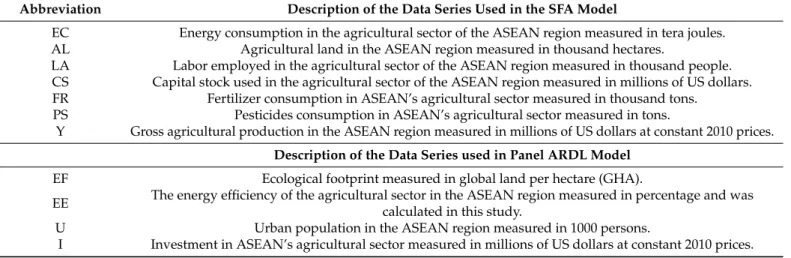
Such factors faster the economic activities such as expansion of industrial zones, high traffic, higher levels of various pollutions. Most of the times, urbanization causes greater environmental contamination [45]. Investment is mostly used as proxy of Research and Development (R&D). R&D strengthens the production techniques through inventions and innovations. In the recent era, before introducing any modern technology, scientists and researchers take under consideration its environmental effects. That is why every modern and advanced strategy becomes more environment friendly. Recently, electricity-based machinery and vehicles are introduced to control the environmental degradation. Table1 presents the descriptions of the data sets used in this study.
Table 1.Description of the data series used in this study.
Abbreviation Description of the Data Series Used in the SFA Model
EC Energy consumption in the agricultural sector of the ASEAN region measured in tera joules.
AL Agricultural land in the ASEAN region measured in thousand hectares.
LA Labor employed in the agricultural sector of the ASEAN region measured in thousand people.
CS Capital stock used in the agricultural sector of the ASEAN region measured in millions of US dollars.
FR Fertilizer consumption in ASEAN’s agricultural sector measured in thousand tons.
PS Pesticides consumption in ASEAN’s agricultural sector measured in tons.
Y Gross agricultural production in the ASEAN region measured in millions of US dollars at constant 2010 prices.
Description of the Data Series used in Panel ARDL Model EF Ecological footprint measured in global land per hectare (GHA).
EE The energy efficiency of the agricultural sector in the ASEAN region measured in percentage and was calculated in this study.
U Urban population in the ASEAN region measured in 1000 persons.
I Investment in ASEAN’s agricultural sector measured in millions of US dollars at constant 2010 prices.
Source: [37,46–48].
This study adopted a stochastic frontier analysis (SFA) approach developed by [35]
to calculate the energy efficiency of the agricultural sector in the ASEAN region. The energy efficiency value is between 0 and 1. The highest EE value shows the efficient use of energy in the agricultural sector. This study transformed the Shephard distance function
(followed by the linear homogeneity property) into an estimated stochastic frontier model for calculating energy efficiency [49]. Equation (1) represents the stochastic frontier distance function [8]:
LnDE(ALit,LAit,CSit,FRit,PSit,ECit,Yit) =α0+α1LnALit+α2LnLAit+α3LnCSit+α4LnFRit+ α5LnPSit+α6LnECit+α7LnYit+α8Lnt+12α11(LnALit)2+12α22(LnLAit)2+12α33(LnCSit)2+
1
2α44(LnFRit)2+12α55(LnPSit)2+12α66(LnECit)2+12α77(LnYit)2+12α88(t)2+α12LnALitLnLAit+ α13LnALitLnCSit+α14LnALitLnFRit+α15LnALitLnPSit+α16LnALitLnECit+α17LnALitLnYit+ α18LnALitLnt+α23LnLAitLnCSit+α24LnLAitLnFRit+α25LnLAitLnPSit+α26LnLAitLnECit+
α27LnLaitLnYit+α28LnLAitLnt+α34LnCSitLnFRit+α35LnCSitLnPSit+α36LnCSitLnECit+ α37LnCSitLnYit+α38LnCSitLnt+α45LnFRitLnPSit+α46LnFRitLnECit+α47LnFRitLnYit+α48LnFRitLnt+
α56LnPSitLnECit+α57LnPSitLnYit+α58LnPSitLnt+α67LnECitLnYit+α78LnYLnt+vit
(1)
Since the input distance function is homogeneous of degree one in inputs, then, dividing the left side, as well as all input variables on the right side, by the amount of energy consumed in agriculture (EC). We have the following equation:
LnDE
ALit,LAit,CSit,FRit,PSit,ECit,Yit
ECit
=α0+α1Ln
ALit
ECit
+α2Ln
LAit
ECit
+α3Ln
CSit
ECit
+α4Ln
FRit
ECit
+α5Ln
PSit
ECit
+ α7LnYit+α8t+12α11
Ln
ALit
ECit
2
+12α22
Ln
LAit
ECit
2
+12α33
Ln
CSit
ECit
2
+12α44
Ln
FRit
ECit
2
+
1 2α55
Ln
PSit
ECit
2
+12α77(LnYit)2+12α88(t)2+α12Ln
ALit
ECit
Ln
LAit
ECit
+α13Ln
ALit
ECit
Ln
CSit
ECit
+ α14Ln
ALit
ECit
Ln
FRit
ECit
+α15Ln
ALit
ECit
Ln
PSit
ECit
+α17Ln
ALit
ECit
LnYit+α18Ln
ALit
ECit
(t) +α23Ln
LAit
ECit
Ln
CSit
ECit
+
α24Ln
LAit
ECit
Ln
FRit
ECit
+α25Ln
LAit
ECit
Ln
PSit
ECit
+α27Ln
LAit
ECit
LnYit+α28Ln
LAit
ECit
(t)+
α34Ln
CSit
ECit
Ln
FRit
ECit
+α35Ln
CSit
ECit
Ln
PSit
ECit
+α37Ln
CSit
ECit
LnYit+α38Ln
CSit
ECit
(t)+
α45Ln
FRit
ECit
Ln
PSit
ECit
+α47Ln
FRit
ECit
LnYit+α48Ln
FRit
ECit
(t) +α57
PSit
ECit
LnYit+α58 PSit
ECit
(t) +vit
(2)
whereDE reveals the distance function,αshows the parameters andvit represents the two-sided random error term considered independent and identically distributed (iid.) N(0,δ2v). The Shephard distance function is linearly homogeneous [50]; Equation (2) is rearranged as:
Ln(1/ECit) =α0+α1Ln
ALit
ECit
+α2Ln
LAit
ECit
+α3Ln
CSit
ECit
+α4Ln
FRit
ECit
+α5Ln
PSit
ECit
+α7LnYit+α8t+
1 2α11
Ln
ALit
ECit
2
+12α22Ln
LAit
ECit
2
+12α33Ln
CSit
ECit
2
+12α44Ln
FRit
ECit
2
+12α55Ln
PSit
ECit
2
+
1
2α77(LnYit)2+12α88(t)2+α12Ln
ALit
ECit
Ln
LAit
ECit
+α13Ln
ALit
ECit
Ln
CSit
ECit
+α14Ln
ALit
ECit
Ln
FRit
ECit
+ α15Ln
ALit
ECit
Ln
PSit
ECit
+α17Ln
ALit
ECit
LnYit+α18Ln
ALit
ECit
(t) +α23Ln
LAit
ECit
Ln
CSit
ECit
+ α24Ln
LAit
ECit
Ln
FRit
ECit
+α25Ln
LAit
ECit
Ln
PSit
ECit
+α27Ln
LAit
ECit
LnYit+α28Ln
LAit
ECit
(t)+
α34Ln
CSit
ECit
Ln
FRit
ECit
+α35Ln
CSit
ECit
Ln
PSit
ECit
+α37Ln
CSit
ECit
LnYit+α38Ln
CSit
ECit
(t)+
α45Ln
FRit
ECit
Ln
PSit
ECit
+α47Ln
FRit
ECit
LnYit+α48Ln
FRit
ECit
(t) +α57PSECit
it
LnYit+α58ECPSit
it
(t) +vit−uit
(3)
Equation (3) is estimated using the maximum likelihood (ML) time-varying efficiency decay model introduced by [51]. Where, uit = e−η(t−T)ui and follows a truncated normal distribution, N µ, δu2
;η is an unknown scalar parameter and indicates time- varying technical inefficiency;tprovides a set of time span between periods T andvit−uit
illustrates the residuals. Thus, in the model, time-varying efficiency is considered to follow an exponential function of time and contains only a single parameter which must be computed. Whenη> 0 then technical inefficiency increases at a decreasing rate or decreases at an increasing rate whenη< 0, and ifηis equal to zero then the time invariant model is obtained. The likelihood function is illustrated in terms ofδ2 = δ2v+δ2u and θ=δ2u/(δ2v+δ2u). Where,θindicates the contribution ofu(variance) to the residual; where,
θ=δ2u/δ2,δ2=δ2v+δ2u, andθe[0, 1]. Therefore, the energy efficiency (EE) forith country at timetcan be calculated using Equation (4):
EEit=E[exp(−uit)] (4) This paper employed a dynamic panel heterogeneity model developed by [41,52].
Panel Autoregressive Distributed Lag (ARDL) model was employed to explore long-run and short-run influence of energy efficiency and other control factors on ecological footprint.
In addition, the panel ARDL model also determines the speed of convergence towards dynamic equilibrium. The time series number is relatively larger than the cross section (T > N). In such state, [53] declared traditional panel approaches such as fixed effect, instrumental variables, and GMM estimators as inconsistent and potentially misleading, unless the slopes are identical. Second, the data series are tested for unit root to ensure robustness or stationarity of the data. Non-stationary data causes spurious regression that is not considered reliable and predictable [54]. The Levin and Lin unit root test (LL test) developed by [55] was applied to examine the unit root problem in the data series.
Equation (5) denotes the general form of the LL test with the intercept term.
∆Sit =a0+ØSit−1+
∑
p i=1βi∆Sit−i+eit (5)
whereSrepresents any variable,a0denotes individual intercept, Ø indicates the slope coefficient of the variableSandeitrepresents residuals at timetwithicross-sections. After unit root analysis, the paper has employed the following panel ARDL model (p,q) based on the following specification [52]:
LnEFit =
∑
p i=1€ijelection criteria ture Ln EFj,t−i +
∑
q j=0£ijLn Ti,t−j
+µi+eit (6)
where,EFandTare exogenous and indigenous factors. Dynamic heterogeneity in panel regression can be added to an error correction model using a panel ARDL (p,q) technique by subtracting the lagged dependent variable (energy efficiency) on both sides as follows:
∆LnEFit =øiLn(EFi,t−1) +∂iLn(Ti,t−1) +
p−1
∑
j=1
∆€ijelection criteria ture Ln EFi,t−j +
q−1
∑
j=0
∆£ijLn Ti,t−j
+µi+eit (7)
where,EFis ecological footprint,Tindicates list of independent variables.€and £ repre- sent the short-run coefficients, and ø and∂are long-run coefficients as well as speed of adjustment towards equilibrium, respectively.µis a country-specific intercept. Further- more, PMG estimator imposes a constraint of homogeneity in the long run among counties, while containing heterogeneity in the short run. Therefore, MG has no such restriction.
Its coefficients can be heterogeneous in the short and long runs. However, [52] analyzed that PMG estimator provides higher efficiency estimates than MG estimator under long run homogeneity. This study employed the Hausman test [56] to determine the most appropriate estimator among pooled mean group (PMG) and mean group (MG) under panel ARDL model. The null hypothesis, H0: the PMG estimator is consistent and efficient estimator, against the alternative hypothesis, H1: MG estimator is consistent and efficient estimator. When the null hypothesis (H0) is accepted against the alternative hypothesis (H1), then PMG is the most efficient and consistent estimator [57].
Equation (8) represents the specification of panel ARDL model [41,52].
∆LnEFit =βo+ ∑a
e=1
β1e election criteria ture∆LnEFit−e+ ∑b
f=1
β2f∆LnEEit−f+ ∑d
h=1
β3h∆LnUit−h
+ ∑e
k=1
β4k∆LnIit−k+δ1LnEFit−1+δ2LnEEit−1+δ3LnUit−1+δ4LnIit−1+δ5ECTit−1+eit
(8)
where,∆represents the difference operator;βandδdenote parameters in the short and long-run, andeitdenotes residual oficross-sections at timet. The termECTit−1indicates the error correction term that determines the dynamic stability of the model. This term relates to the fact that the deviation of the last period from a long-term equilibrium, the error, influences its short-term dynamics. In addition, the error correction term shows the long run relationship [58,59].
3. Results and Discussion
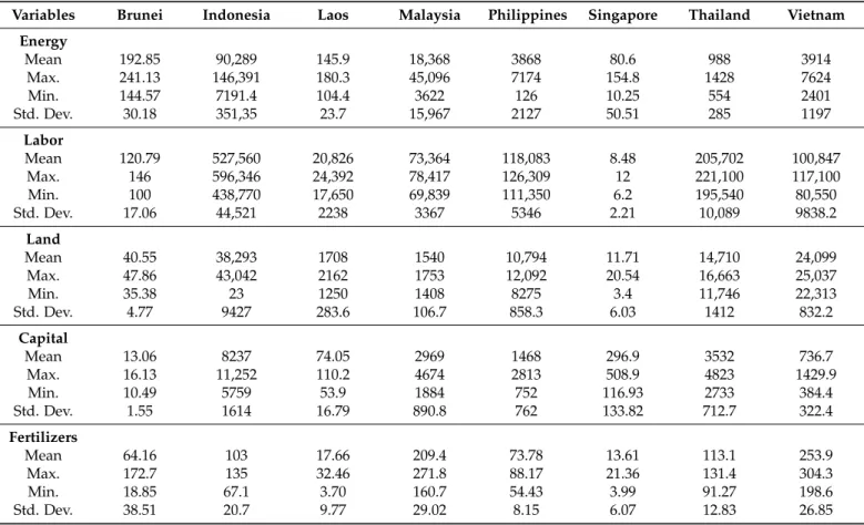
This paper explored the impact of energy efficiency on ecological footprint in the ASEAN region. Table2presents descriptive statistics of seven data series used in this study to calculate energy efficiency. These include energy consumption, agricultural land, labor employed in agriculture, capital stock, consumption of fertilizers, use of pesticides, and gross agricultural production. Each data series presents an average value followed by its maximum, minimum value, and standard deviation. Regression reliability and stability superficially depend on the basic data statistics. These also provide an overview of data collected from various data sources. An experienced reader can easily distinguish original and false data by reviewing descriptive statistics. In Table2, the mean value represents an average value of the data that resides mainly in the middle part of the data. Maximum and minimum are basically the data range where all data values must fall between these two upper and lower limits. The standard deviation indicates the dispersion of the data values from their meander or center value. Very high standard deviation values are not recognized as good for analysis because high standard deviation values lead to the outlier problem. By analyzing the descriptive statistics, it can be understood that the data obtained in this study are normally distributed and free from other problems. In addition, the data is reliable, predictable, and stable, and it is perfect for analysis [60].
Table 2.Descriptive statistics of the data series used to calculate energy efficiency.
Variables Brunei Indonesia Laos Malaysia Philippines Singapore Thailand Vietnam Energy
Mean 192.85 90,289 145.9 18,368 3868 80.6 988 3914
Max. 241.13 146,391 180.3 45,096 7174 154.8 1428 7624
Min. 144.57 7191.4 104.4 3622 126 10.25 554 2401
Std. Dev. 30.18 351,35 23.7 15,967 2127 50.51 285 1197
Labor
Mean 120.79 527,560 20,826 73,364 118,083 8.48 205,702 100,847
Max. 146 596,346 24,392 78,417 126,309 12 221,100 117,100
Min. 100 438,770 17,650 69,839 111,350 6.2 195,540 80,550
Std. Dev. 17.06 44,521 2238 3367 5346 2.21 10,089 9838.2
Land
Mean 40.55 38,293 1708 1540 10,794 11.71 14,710 24,099
Max. 47.86 43,042 2162 1753 12,092 20.54 16,663 25,037
Min. 35.38 23 1250 1408 8275 3.4 11,746 22,313
Std. Dev. 4.77 9427 283.6 106.7 858.3 6.03 1412 832.2
Capital
Mean 13.06 8237 74.05 2969 1468 296.9 3532 736.7
Max. 16.13 11,252 110.2 4674 2813 508.9 4823 1429.9
Min. 10.49 5759 53.9 1884 752 116.93 2733 384.4
Std. Dev. 1.55 1614 16.79 890.8 762 133.82 712.7 322.4
Fertilizers
Mean 64.16 103 17.66 209.4 73.78 13.61 113.1 253.9
Max. 172.7 135 32.46 271.8 88.17 21.36 131.4 304.3
Min. 18.85 67.1 3.70 160.7 54.43 3.99 91.27 198.6
Std. Dev. 38.51 20.7 9.77 29.02 8.15 6.07 12.83 26.85
Table 2.Cont.
Variables Brunei Indonesia Laos Malaysia Philippines Singapore Thailand Vietnam Pesticides
Mean 1.09 0.03 0.58 6.62 0.24 5.85 2.33 2.02
Max. 3.85 0.05 0.93 8.47 0.97 8.4 4.72 2.81
Min. 0.16 0.03 0.41 5.74 0.03 4.1 0.38 1.66
Std. Dev. 1.01 0.01 0.15 0.98 0.23 1.44 1.25 0.24
Production
Mean 98.78 97,500 1460 23,800 22,900 95.05 34,100 19,700
Max. 117 133,000 1900 29,300 26,700 127 39,500 25,200
Min. 67.86 719,000 1130 18,100 16,400 79.72 25,900 13,800
Std. Dev. 13.45 19,600 250 3850 3270 14.77 4070 3640
Source: [37,46–48].
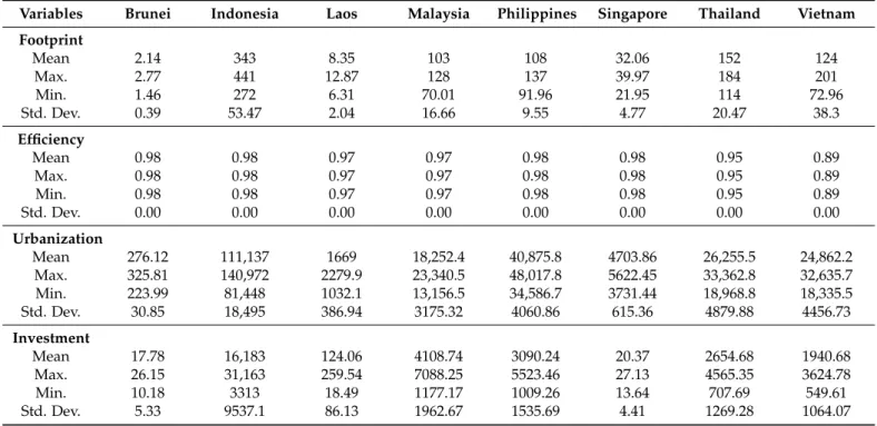
Table3presents descriptive statistics of the variables used in the panel ARDL model.
These data series are ecological footprint, energy efficiency, urbanization, and investment in agricultural sector. Each data series provides the average value followed by its maximum, minimum value, and standard deviation. Descriptive statistics of the dependent and independent variables used in the panel ARDL model also show that these variables are reliable, stable, and predictable, and practical decisions can be made based on their regression results.
Table 3.Descriptive statistics of the variable used in the panel ARDL model.
Variables Brunei Indonesia Laos Malaysia Philippines Singapore Thailand Vietnam Footprint
Mean 2.14 343 8.35 103 108 32.06 152 124
Max. 2.77 441 12.87 128 137 39.97 184 201
Min. 1.46 272 6.31 70.01 91.96 21.95 114 72.96
Std. Dev. 0.39 53.47 2.04 16.66 9.55 4.77 20.47 38.3
Efficiency
Mean 0.98 0.98 0.97 0.97 0.98 0.98 0.95 0.89
Max. 0.98 0.98 0.97 0.97 0.98 0.98 0.95 0.89
Min. 0.98 0.98 0.97 0.97 0.98 0.98 0.95 0.89
Std. Dev. 0.00 0.00 0.00 0.00 0.00 0.00 0.00 0.00
Urbanization
Mean 276.12 111,137 1669 18,252.4 40,875.8 4703.86 26,255.5 24,862.2
Max. 325.81 140,972 2279.9 23,340.5 48,017.8 5622.45 33,362.8 32,635.7
Min. 223.99 81,448 1032.1 13,156.5 34,586.7 3731.44 18,968.8 18,335.5
Std. Dev. 30.85 18,495 386.94 3175.32 4060.86 615.36 4879.88 4456.73
Investment
Mean 17.78 16,183 124.06 4108.74 3090.24 20.37 2654.68 1940.68
Max. 26.15 31,163 259.54 7088.25 5523.46 27.13 4565.35 3624.78
Min. 10.18 3313 18.49 1177.17 1009.26 13.64 707.69 549.61
Std. Dev. 5.33 9537.1 86.13 1962.67 1535.69 4.41 1269.28 1064.07
Source: [37,46–48].
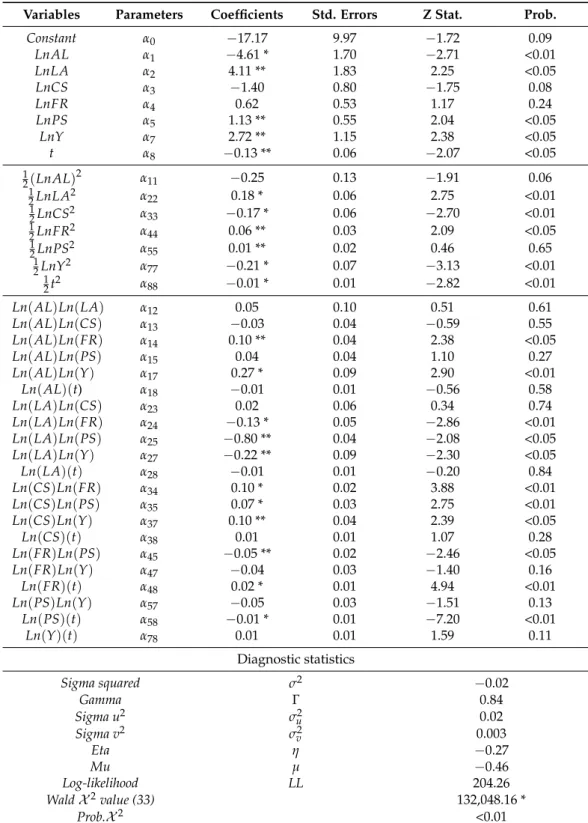
Table4presents the findings of ML time-varying efficiency decay model developed by [61]. The calculated value of Log-likelihood (LL) is 204.26 and exceeds the critical value at 1%. This explored that the agricultural sector in the ASEAN region is inefficient in terms of energy use. The parameters (σ2u,σ2v) were transformed into (σ2,γ) withσ2=σ2u+σ2vand γ=σ2u/σ2[51]. Theγvalue is a significant part of the composite error [62] and captures the inefficiency in the use of energy in the agricultural sector. The higher the value ofγ, the greater the inefficiency in the use of energy. Theγvalue is 0.84 and shows that 84%
of the total variability in gross agricultural production in the ASEAN region was due to
the inefficient use of energy. In addition, technical inefficiency in the ASEAN rural sector decreases at an increasing rate asηis less than zero, that is,−0.27.
Table 4.Results of ML time-varying efficiency decay model.
Variables Parameters Coefficients Std. Errors Z Stat. Prob.
Constant α0 −17.17 9.97 −1.72 0.09
LnAL α1 −4.61 * 1.70 −2.71 <0.01
LnLA α2 4.11 ** 1.83 2.25 <0.05
LnCS α3 −1.40 0.80 −1.75 0.08
LnFR α4 0.62 0.53 1.17 0.24
LnPS α5 1.13 ** 0.55 2.04 <0.05
LnY α7 2.72 ** 1.15 2.38 <0.05
t α8 −0.13 ** 0.06 −2.07 <0.05
1
2(LnAL)2 α11 −0.25 0.13 −1.91 0.06
1
2LnLA2 α22 0.18 * 0.06 2.75 <0.01
1
2LnCS2 α33 −0.17 * 0.06 −2.70 <0.01
1
2LnFR2 α44 0.06 ** 0.03 2.09 <0.05
1
2LnPS2 α55 0.01 ** 0.02 0.46 0.65
12LnY2 α77 −0.21 * 0.07 −3.13 <0.01
1
2t2 α88 −0.01 * 0.01 −2.82 <0.01
Ln(AL)Ln(LA) α12 0.05 0.10 0.51 0.61
Ln(AL)Ln(CS) α13 −0.03 0.04 −0.59 0.55
Ln(AL)Ln(FR) α14 0.10 ** 0.04 2.38 <0.05
Ln(AL)Ln(PS) α15 0.04 0.04 1.10 0.27
Ln(AL)Ln(Y) α17 0.27 * 0.09 2.90 <0.01
Ln(AL)(t) α18 −0.01 0.01 −0.56 0.58
Ln(LA)Ln(CS) α23 0.02 0.06 0.34 0.74
Ln(LA)Ln(FR) α24 −0.13 * 0.05 −2.86 <0.01
Ln(LA)Ln(PS) α25 −0.80 ** 0.04 −2.08 <0.05
Ln(LA)Ln(Y) α27 −0.22 ** 0.09 −2.30 <0.05
Ln(LA)(t) α28 −0.01 0.01 −0.20 0.84
Ln(CS)Ln(FR) α34 0.10 * 0.02 3.88 <0.01
Ln(CS)Ln(PS) α35 0.07 * 0.03 2.75 <0.01
Ln(CS)Ln(Y) α37 0.10 ** 0.04 2.39 <0.05
Ln(CS)(t) α38 0.01 0.01 1.07 0.28
Ln(FR)Ln(PS) α45 −0.05 ** 0.02 −2.46 <0.05
Ln(FR)Ln(Y) α47 −0.04 0.03 −1.40 0.16
Ln(FR)(t) α48 0.02 * 0.01 4.94 <0.01
Ln(PS)Ln(Y) α57 −0.05 0.03 −1.51 0.13
Ln(PS)(t) α58 −0.01 * 0.01 −7.20 <0.01
Ln(Y)(t) α78 0.01 0.01 1.59 0.11
Diagnostic statistics
Sigma squared σ2 −0.02
Gamma Γ 0.84
Sigma u2 σu2 0.02
Sigma v2 σv2 0.003
Eta η −0.27
Mu µ −0.46
Log-likelihood LL 204.26
WaldX2value (33) 132,048.16 *
Prob.X2 <0.01
* 1% level of significance, ** 5% level of significance.
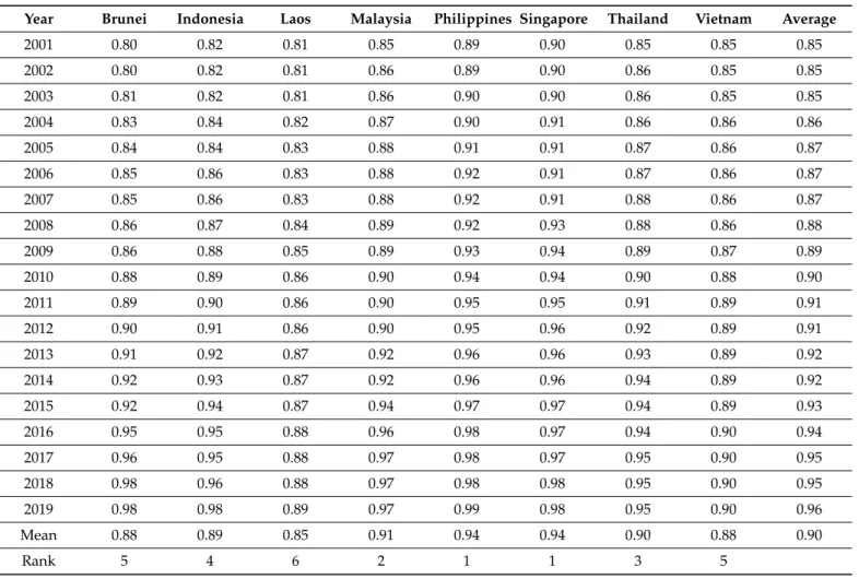
Table5describes the energy efficiency scores of the agricultural sector in the ASEAN region. Based on average efficiency scores, the Philippines and Singapore are the most energy efficient economies, with efficiency scores of 94% each. This indicates that both economies consist of strong and efficient production systems. They mainly use advanced and improved production technologies. Because they have a strong efficiency score, their
production cost is close to the lowest level. Furthermore, the efficient allocation of energy resources leads to the strengthening of their economic growth and development. Therefore, there is still an ideal space to further improve their energy efficiency by 6%. Laos is the most energy-inefficient economy in the ASEAN region, with an efficiency score of 85%
ranging from 81% to 89%. In addition, there is still 15% room for improvement in the energy efficiency of the agricultural sector in Laos. The results reveal that Laos is somewhat weak in its production performance as compared to other countries in the ASEAN region.
The average efficiency score of the ASEAN region is around 90%, ranging from 85% to 96%. Therefore, there is still 10% room for improvement in energy efficiency. In addition, energy efficiency of the agricultural sector in ASEAN countries shows an increasing trend.
Furthermore, the highest efficiency score (96%) in the ASEAN region was recorded in 2019.
Figure1also shows the trend of energy efficiency in ASEAN countries.
Table 5.The trend of energy efficiency in ASEAN countries.
Year Brunei Indonesia Laos Malaysia Philippines Singapore Thailand Vietnam Average
2001 0.80 0.82 0.81 0.85 0.89 0.90 0.85 0.85 0.85
2002 0.80 0.82 0.81 0.86 0.89 0.90 0.86 0.85 0.85
2003 0.81 0.82 0.81 0.86 0.90 0.90 0.86 0.85 0.85
2004 0.83 0.84 0.82 0.87 0.90 0.91 0.86 0.86 0.86
2005 0.84 0.84 0.83 0.88 0.91 0.91 0.87 0.86 0.87
2006 0.85 0.86 0.83 0.88 0.92 0.91 0.87 0.86 0.87
2007 0.85 0.86 0.83 0.88 0.92 0.91 0.88 0.86 0.87
2008 0.86 0.87 0.84 0.89 0.92 0.93 0.88 0.86 0.88
2009 0.86 0.88 0.85 0.89 0.93 0.94 0.89 0.87 0.89
2010 0.88 0.89 0.86 0.90 0.94 0.94 0.90 0.88 0.90
2011 0.89 0.90 0.86 0.90 0.95 0.95 0.91 0.89 0.91
2012 0.90 0.91 0.86 0.90 0.95 0.96 0.92 0.89 0.91
2013 0.91 0.92 0.87 0.92 0.96 0.96 0.93 0.89 0.92
2014 0.92 0.93 0.87 0.92 0.96 0.96 0.94 0.89 0.92
2015 0.92 0.94 0.87 0.94 0.97 0.97 0.94 0.89 0.93
2016 0.95 0.95 0.88 0.96 0.98 0.97 0.94 0.90 0.94
2017 0.96 0.95 0.88 0.97 0.98 0.97 0.95 0.90 0.95
2018 0.98 0.96 0.88 0.97 0.98 0.98 0.95 0.90 0.95
2019 0.98 0.98 0.89 0.97 0.99 0.98 0.95 0.90 0.96
Mean 0.88 0.89 0.85 0.91 0.94 0.94 0.90 0.88 0.90
Rank 5 4 6 2 1 1 3 5
Source: Authors’ calculation.
Figure 1.The trend of energy efficiency in ASEAN countries.
Table6presents the results of the panel unit root based on the Levin Lin test [55]. The results show that the energy efficiency (EE) and ecological footprint (EE) data series are stationary at first difference i.e., I (1) and urbanization (U) and investment in agriculture (I) are stationary at level i.e., I (0).
Table 6.Results of Levin Lin (LL) test.
Variables tStat. pValue Bandwidth Conclusion
LnEF −1.30 0.90 (2)
∆LnEF −1.94 ** <0.05 (4) I (1)
LnEE −1.21 0.66 (1)
∆LnEE −3.98 * <0.01 (1) I (1)
LnU −6.82 * <0.01 (2) I (0)
∆LnU - - -
LnI −3.93 * <0.01 (2) I (0)
∆LnI - - -
* 1% level of significance, ** 5% level of significance.
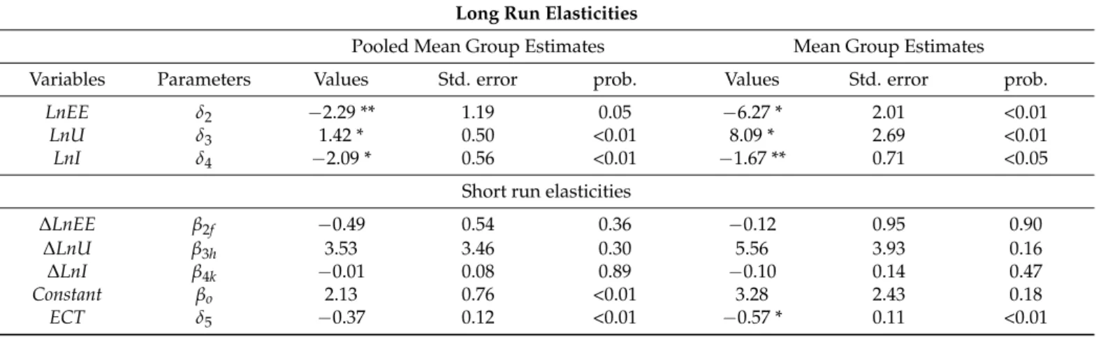
Finally, this study applied the panel ARDL model to examine the long and short-run impact of energy efficiency on the ecological footprint in the ASEAN region. Table7reports the results based on the pooled mean group (PMG) and mean group (MG) estimators for the ARDL model. From these results, the MG was estimated from the country without restrictions by country estimate. The coefficients of the MG estimator are the mean of the country-specific parameters and the PMG coefficients are restricted to be the same
across the countries. Thus, the comparison between the results of the PMG (long-term slope homogeneity) and MG (long-term slope homogeneity) estimates shows how the empirical estimates of the efficiency model are sensitive to different estimation techniques.
This study applied the Hausman test [56] to test whether there is a significant difference between the PMG and MG estimators. Where, under the null hypothesis, the difference in the estimated coefficients between the MG and the PMG are not significantly different i.e., the PMG is more efficient. The estimated value of the Hausman test that follows the Chi-square distribution is 1.40, which is not statistically significant at 5%. We accept the null hypothesis and conclude that the PMG estimator is preferred. The pooled mean group has advantages in determining dynamic long- and short-run relationships.
Table 7.Findings of the pooled mean group (PMG) and mean group (MG).
Long Run Elasticities
Pooled Mean Group Estimates Mean Group Estimates
Variables Parameters Values Std. error prob. Values Std. error prob.
LnEE δ2 −2.29 ** 1.19 0.05 −6.27 * 2.01 <0.01
LnU δ3 1.42 * 0.50 <0.01 8.09 * 2.69 <0.01
LnI δ4 −2.09 * 0.56 <0.01 −1.67 ** 0.71 <0.05
Short run elasticities
∆LnEE β2f −0.49 0.54 0.36 −0.12 0.95 0.90
∆LnU β3h 3.53 3.46 0.30 5.56 3.93 0.16
∆LnI β4k −0.01 0.08 0.89 −0.10 0.14 0.47
Constant βo 2.13 0.76 <0.01 3.28 2.43 0.18
ECT δ5 −0.37 0.12 <0.01 −0.57 * 0.11 <0.01
Note: * and ** indicate 1% & 5% significance level, respectively.
The results show that energy efficiency, urbanization, and investment have a strong relationship with ecological footprint in the long run. Based on the findings, the efficient implementation of energy sources in ASEAN’s rural sector will reduce environmental contamination, especially in the long run. It is supporting the argument that advanced energy sources reduce greenhouse gas emissions in agriculture, which is beneficial to the environment [24,63–69]. The tendency of people towards cities is not a problem in the short run, so in the long run, it significantly increases the ecological footprint. It is due to the increased spending of areas of the city for consumption purposes. In addition, congested cities need considerable land and other resources to protect the environment from further degradation [7,70]. Investment in the agricultural sector is a significant factor that reduces the ecological footprint in the long run. Investment is mainly used to implement modern agricultural practices, which [67] are also a significant determinant of energy efficiency.
The investment encourages farmers to use machines with low fuel consumption in the cultivation process. The investment also allows the use of electricity in agriculture, which has been considered one of the most ecological agricultural inputs [71]. In addition, the error correction term (ECT) represents that the model is dynamically stable, which removes the short-run imbalance in the long run. Dynamic stability consists of two assumptions, the ECT coefficient must be negative and significant. In the conclusions, the value of the coefficient of the error correction term is−0.37. clearly satisfies the first assumption of having a negative ECT coefficient. and is significant at 1%. Thus, it is concluded that the estimated panel ARDL model is dynamically stable with an adjustment effect of 37% per year. It illustrates that the short-term imbalance will automatically adjust over the next 2.7 years [72–74].
Under the homogeneity of the long-run slope, Hausman’s statistic is asymptotically distributed as a chi-square with three degrees of freedom [75]. The lag structure is ARDL (1,1,1,1,1).
Two-way causality is an inherent aspect of any robust policy design, and a comprehen- sive policy framework must take this specific aspect into account. Therefore, following the literature [76] to obtain additional information on the directional nature of the associations between the model parameters, we used the paired-panel Granger causality test [77]. The results of paired-panel Granger causality are reported in Table8The results of the paired wise panel Granger causality test show that energy efficiency, urbanization, and investment in agriculture cause ecological footprint. Further findings reveal a unidirectional causality from energy efficiency, urbanization, and investment in agriculture to ecological footprint.
These findings are consistent with the results of [78]. Finally, the model diagnostic statistics are provided in Table9.
Table 8.Results of panel causality test.
Causality Direction Test Statistics Causality Direction Test Statistics
EE→EF 6.18 * EF→EE 0.63
U→EF 3.56 ** EF→U 0.04
I→EF 4.39 * EF→I 0.59
* 1% level of significance, ** 5% level of significance.
Table 9.Results of diagnostic tests of the panel ARDL model.
Diagnostic Tests Test Statistics
Hausman test 1.40 (0.84)
Normality 0.90 (0.62)
Omitted Variable Bias 1.3 (0.51)
Note:p-values are within parentheses.
4. Conclusions and Policy Implications
The objectives of this study are twofold: first, this study technically calculated energy efficiency of the agricultural sector in ASEAN countries and then investigated the effect of technically derived energy efficiency on the ecological footprint. Several methodologies were employed to achieve the basic objective of this study. The results of the stochastic frontier analysis showed that the interaction effects between the agricultural inputs are common in the agricultural sector. In addition, the results of stochastic frontier analysis explored that the average efficiency score of the agricultural sector in the ASEAN coun- tries is around 90%, ranging from 85% to 96%. and shows that there is still 10% room for improvement in energy efficiency of agricultural sector in the ASEAN region. The Philippines and Singapore were the most energy efficient economies; Laos is the least energy efficient country as compared to other countries in the ASEAN region. The LL analysis shows that ecological footprint (EF) and energy efficiency (EE) are stationary at first difference, while urbanization (U) and investment (I) are stationary at level. The results of the PMG of the panel ARDL model show that energy efficiency and investment in the agricultural sector are beneficial for the environment in the long run. In addition, this study concludes that energy efficiency, urbanization, and investment in agriculture are long-run phenomena. Urbanization is also a growing factor in the ecological footprint. The ECT term also confirmed that the panel ARDL model is dynamic stability in the long run.
Finally, several policy implications were conceived based on the findings of this study in general and particularly for ASEAN countries: (1) The study found that efficient use of energy in agriculture reduces the environmental impact. Therefore, this study suggests that energy efficient agricultural technologies should be introduced or enhanced in the agricultural sector of the ASEAN region. This will reduce the cost of agricultural pro- duction and consequently reduce ecological footprint and environmental contaminations.
(2) The results of this study also recommend that urbanization increases the ecological footprint and deteriorates environmental quality. One of the main factors encouraging rural-urban migration in the ASEAN region is the low standard of living and the scarcity of necessary amenities in rural areas. As a result, people move from rural to urban in the
ASEAN countries to improve their quality of life. Therefore, this study suggests that the government and other stakeholders in this region should provide the necessary amenities for the rural population, and this will help to curb rural–urban migration and reduce environmental degradation in the ASEAN region. (3) Finally, this study also explored that investment in agriculture plays a significant role in reducing the ecological footprint and, consequently, environmental containments. Therefore, the ASEAN region should place greater emphasize on investments in agriculture through public–private partnerships. This will increase agricultural productivity on one hand and reduce the ecological footprint and environmental containments on the other.
Author Contributions:Conceptualization, D.K. and M.N.; methodology, J.P.; software, M.N.; valida- tion, D.K., M.N. and M.A.K.; formal analysis, M.N.; investigation, F.U.R.; resources, J.P.; data curation, M.N. and F.U.R.; writing—original draft preparation, M.N., D.K. and F.U.R.; writing—review and editing, J.O.; visualization, J.P.; supervision, D.K. and M.A.K.; project administration, F.U.R. and M.A.K.; funding acquisition, J.P. and J.O. All authors have read and agreed to the published version of the manuscript.
Funding: Project no. 132805 has been implemented with support provided from the National Research, Development, and Innovation Fund of Hungary, financed under the K_19 funding scheme and supported by the János Bolyai Research Scholarship of the Hungarian Academy of Sciences (BO/00095/18 and BO/8/20).
Data Availability Statement:World Data is openly accessed and freely available to everyone.
Conflicts of Interest:The authors declare no conflict of interest.
References
1. Kijima, M.; Nishide, K.; Ohyama, A. Economic models for the environmental Kuznets curve: A survey.J. Econ. Dyn. Control2010, 34, 1187–1201. [CrossRef]
2. Shahbaz, M.; Hye, Q.M.A.; Tiwari, A.K.; Leitão, N.C. Economic growth, energy consumption, financial development, international trade and CO2emissions in Indonesia.Renew. Sustain. Energy Rev.2013,25, 109–121. [CrossRef]
3. Rees, W.E. Eco-footprint analysis: Merits and brickbats.Ecol. Econ.2000,32, 371–374.
4. Ali, B.; Ullah, A.; Khan, D. Does the prevailing Indian agricultural ecosystem cause carbon dioxide emission? A consent towards risk reduction.Environ. Sci. Pollut. Res.2021,28, 4691–4703. [CrossRef] [PubMed]
5. Herendeen, R.A. Ecological footprint is a vivid indicator of indirect effects.Ecol. Econ.2000,32, 357–358.
6. Simmons, C.; Lewis, K.; Barrett, J. Two feet—Two approaches: A component-based model of ecological footprinting.Ecol. Econ.
2000,32, 375–380.
7. Jorgenson, A.K.; Rice, J.; Crowe, J. Unpacking the ecological footprint of nations.Int. J. Comp. Sociol.2005,46, 241–260. [CrossRef]
8. Shen, X.; Lin, B. Total Factor Energy Efficiency of China’s Industrial Sector: A Stochastic Frontier Analysis.Sustainability2017,9, 646. [CrossRef]
9. Zhao, C.; Zhang, H.; Zeng, Y.; Li, F.; Liu, Y.; Qin, C.; Yuan, J. Total-Factor Energy Efficiency in BRI Countries: An Estimation Based on Three-Stage DEA Model.Sustainability2018,10, 278. [CrossRef]
10. Ullah, A.; Khan, D.; Zheng, S. The determinants of technical efficiency of peach growers: Evidence from Khyber Pakhtunkhwa, Pakistan.Custos E Agronegocio Line2017,13, 211–238.
11. Woods, J.; Williams, A.; Hughes, J.K.; Black, M.; Murphy, R. Energy and the food system.Philos. Trans. R. Soc. B Biol. Sci.2010, 365, 2991–3006. [CrossRef]
12. Miao, C.; Fang, D.; Sun, L.; Luo, Q.; Yu, Q. Driving effect of technology innovation on energy utilization efficiency in strategic emerging industries.J. Clean. Prod.2018,170, 1177–1184. [CrossRef]
13. Nagaoka, S.; Motohashi, K.; Goto, A. Patent statistics as an innovation indicator. InHandbook of the Economics of Innovation;
Elsevier: Amsterdam, The Netherlands, 2010; Volume 2, pp. 1083–1127.
14. Yuan, R.; Li, C.; Li, N.; Khan, M.A.; Sun, X.; Khaliq, N. Can Mixed-Ownership Reform Drive the Green Transformation of SOEs?
Energies2021,14, 2964. [CrossRef]
15. Virglerova, Z.; Khan, M.A.; Martinkute-Kauliene, R.; Kovács, S. The internationalization of SMEs in Central Europe and its impact on their methods of risk management.Amfiteatru Econ.2020,22, 792–807.
16. Kabir, A.; Gilani, S.M.; Rehman, G.; Sabahat, S.H.; Popp, J.; Hassan, M.A.S.; Oláh, J. Energy-aware caching and collaboration for green communication systems.Acta Montan. Slovaca2021,26, 47–59.
17. Virglerova, Z.; Conte, F.; Amoah, J.; Massaro, M.R. The Perception Of Legal Risk And Its Impact On The Business Of Smes.Int. J.
Entrep. Knowl.2020,8, 1–13. [CrossRef]
18. Wu, J.; Xiong, B.; An, Q.; Sun, J.; Wu, H. Total-factor energy efficiency evaluation of Chinese industry by using two-stage DEA model with shared inputs.Ann. Oper. Res.2017,255, 257–276. [CrossRef]
![Table 6 presents the results of the panel unit root based on the Levin Lin test [55]. The results show that the energy efficiency (EE) and ecological footprint (EE) data series are stationary at first difference i.e., I (1) and urbanization (U) and investm](https://thumb-eu.123doks.com/thumbv2/9dokorg/744348.30850/11.892.250.843.859.1021/presents-results-efficiency-ecological-footprint-stationary-difference-urbanization.webp)