A felsőfokú oktatás minőségének és hozzáférhetőségének egÿuttes javı́tása a Pannon Egyetemen
EFOP-3.4.3-16-2016-00009
Introduction to Numerical Analysis Ferenc Hartung
H-8200 Veszpr Egyetem u.10.
H-8201 Veszpr Pf. 158.
Telefon: (+36 88) 624-848 Internet: www.uni-pannon.hu
2018
Table of contents
Table of contents . . . 3
1. Introduction . . . 5
1.1. The Main Objective and Notions of Numerical Analysis . . . 5
1.2. Computer Representation of Integers and Reals . . . 9
1.3. Error Analysis . . . 15
1.4. The Consequences of the Floating Point Arithmetic . . . 18
2. Nonlinear algebraic equations and systems . . . 23
2.1. Review of Calculus . . . 23
2.2. Fixed-Point Iteration . . . 24
2.3. Bisection Method . . . 29
2.4. Method of False Position . . . 30
2.5. Newton’s Method . . . 33
2.6. Secant Method . . . 35
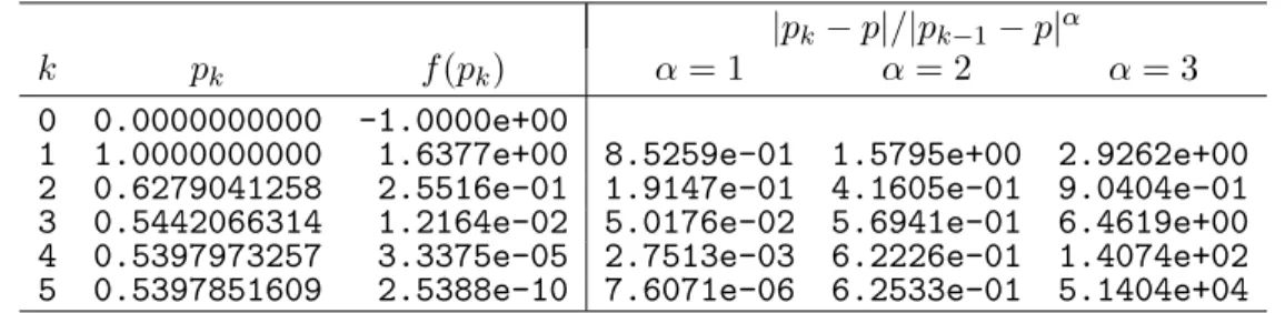
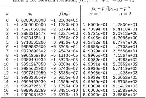
2.7. Order of Convergence . . . 38
2.8. Stopping Criteria of Iterations . . . 44
2.9. Review of Multivariable Calculus . . . 45
2.10. Vector and Matrix Norms and Convergence . . . 47
2.11. Fixed-Point Iteration in n-dimension . . . 54
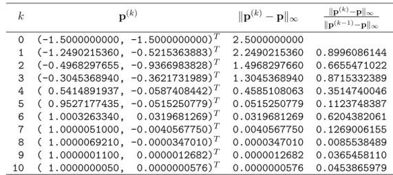
2.12. Newton’s Method in n-dimension . . . 58
2.13. Quasi-Newton Methods, Broyden’s Method . . . 59
3. Linear Systems . . . 65
3.1. Review of Linear Algebra . . . 65
3.2. Triangular Systems . . . 70
3.3. Gaussian Elimination, Pivoting Strategies . . . 71
3.4. Gauss–Jordan Elimination . . . 82
3.5. Tridiagonal Linear Systems . . . 84
3.6. Simultaneous Linear Systems . . . 85
3.7. Matrix Inversion and Determinants . . . 86
4. Iterative Techniques for Solving Linear Systems . . . 89
4.1. Linear Fixed-Point Iteration . . . 89
4.2. Jacobi Iteration . . . 93
4.3. Gauss–Seidel Iteration . . . 96
4.4. Error Bounds and Iterative Refinement . . . 99
4.5. Perturbation of Linear Systems . . . 102
5. Matrix Factorization . . . 107
5.1. LU Factorization . . . 107
5.2. Cholesky Factorization . . . 110
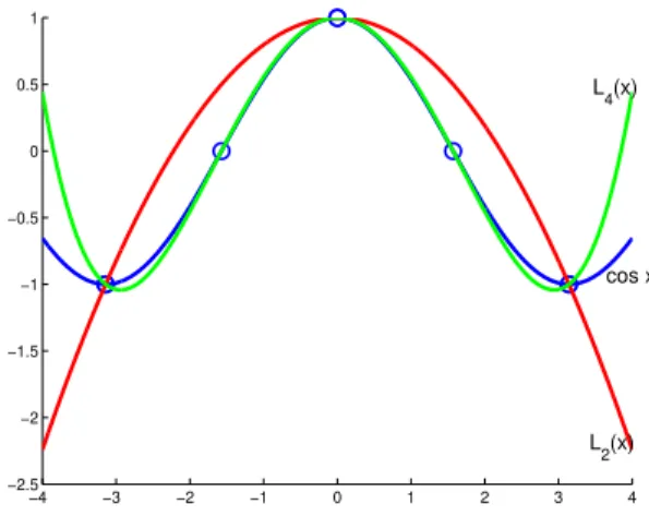
6. Interpolation . . . 113
6.1. Lagrange Interpolation . . . 113
6.2. Divided Differences . . . 119
6.3. Newton’s Divided Difference Formula . . . 121
6.4. Hermite Interpolation . . . 125
6.5. Spline Interpolation . . . 130
7. Numerical Differentiation and Integration . . . 137
7.1. Numerical differentiation . . . 137
7.2. Richardson’s extrapolation . . . 144
7.3. Newton–Cotes Formulas . . . 146
7.4. Gaussian Quadrature . . . 153
8. Minimization of Functions . . . 159
8.1. Review of Calculus . . . 159
8.2. Golden Section Search Method . . . 160
8.3. Simplex Method . . . 163
8.4. Gradient Method . . . 167
8.5. Solving Linear Systems with Gradient Method . . . 170
8.6. Newton’s Method for Minimization . . . 173
8.7. Quasi-Newton Method for Minimization . . . 174
9. Method of Least Squares . . . 183
9.1. Line Fitting . . . 184
9.2. Polynomial Curve Fitting . . . 186
9.3. Special Nonlinear Curve Fitting . . . 189
10. Ordinary Differential Equations . . . 193
10.1. Review of Differential Equations . . . 193
10.2. Euler’s Method . . . 195
10.3. Effect of Rounding in the Euler’s Method . . . 200
10.4. Taylor’s Method . . . 201
10.5. Runge–Kutta Method . . . 203
References. . . 209
Index . . . 211
Chapter 1 Introduction
In this chapter we discuss first the main objectives of numerical analysis and introduce some basic notions. We investigate different sources of errors in scientific computation, define the notion of stability of a mathematical problem or a numerical algorithm, the time and memory resources needed to perform the algorithm. We study the computer representation of integer and real numbers, and present some numerical problems due to the finite-digit arithmetic.
1.1. The Main Objective and Notions of Numerical Analysis
In scientific computations the first step is the mathematical modeling of the physical pro- cess. This is the task of the particular scientific discipline (physics, chemistry, biology, economics, etc.). The resulting model frequently contains parameters, constants, initial data which are typically determined by observations or measurements. If the mathemat- ical model and its parameters are given, then we can use it to answer some questions related to the physical problem. We can ask qualitative questions (Does the problem have a unique solution? Does the solution have a limit as the time goes to infinity? Is the solution periodic? etc.), or we can ask quantitative questions (What is the value of the physical variable at a certain time? What is the approximate solution of the model?).
The qualitative questions are discussed in the related mathematical discipline, but the quantitative questions are the main topics of numerical analysis. The main objective of numerical analysis is to give exact or approximate solutions of a mathematical problem using arithmetic operations (addition, subtraction, multiplication and division). See Fig- ure 1.1 below for the schematic steps of the scientific computation of physical processes.
The numerical value of a physical quantity computed by a process described in Fig- ure 1.1 is, in general, not equal to the real value of the physical quantity. The sources of error we get is divided into the following two main categories: inherited error andcompu- tational error. The mathematical modeling is frequently a simplification of the physical reality, so we generate an inherited error when we replace the physical problem by a mathematical model. This kind of error is called modeling error. An other subclass of the inherited error is what we get when we determine the parameters of the mathematical model by measurements, so we use an approximate parameter value instead of the true one. This is called measurement error.
physical problem
mathematical model - parameters - constants - initial values
numerical solution inherited error:
- modeling error - measurement error
computational error:
- truncation error - rounding error Figure 1.1: Scientific computations
The computational error is divided into two classes: truncation error and rounding error. We get a truncation error when we replace the exact value of a mathematical expression with an approximate formula.
Example 1.1. Suppose we need to compute the value of the functionf(x) = sinxat a certain argument x. We can do it using arithmetic operations if instead of the function value f(x) we compute, e.g., its Taylor-polynomial around 0 of degree 5: T5(x) = x−x3/3! +x5/5!. The Taylor’s theorem (Theorem 2.5 below) says that if f(x) is replaced byT5(x), then the resulting error has the form f(6)6!(ξ)x6 = −sin6!ξx6, where ξ is a number between 0 and x. This is the truncation error of the approximation, which is small if x is close to 0.
□
The rounding error appears since real numbers can be stored in computers with fi- nite digits accuracy. Therefore, we almost always generate a rounding error when we store a real number in a computer. Also, after computing each arithmetic operations, the computer rounds the result to a number which can be stored in the computer (see Sections 1.2–1.4).
When we specify a numerical algorithm, the first thing we have to investigate is the truncation error, since a numerical value is useful only if we know how large is the error of the approximation. The next notion we discuss related to a numerical algorithm is the stability. This notion is used in two meanings in numerics. We can talk about the stability of a mathematical model or about the stability of a numerical method. First we consider an example.
Example 1.2. Consider the linear system
8x+ 917y= 1794 7x+ 802y= 1569.
Its exact solution is x=−5 andy = 2. But if we change the coefficient of the variablex in the second equation to 7.01, then the solution of the corresponding system
1.1. The Main Objective and Notions of Numerical Analysis 7 8x+ 917y= 1794
7.01x+ 802y= 1569
is x=−1.232562589 and y= 1.967132499 (up to 9 decimal digits precision). We observe that 0.14% change in the size of a single coefficient results in 75.3% and 1.6% changes in the solutions,
rspectively.
□
We say that a mathematical problem is correct or stable or well-conditioned, if a
“small” change in the parameters of the problem results only in “small” change in the solution of the problem. In the opposite case we say that the problem is incorrect or ill-conditioned or unstable problem. The linear system in the previous example is an incorrect mathematical problem.
We say that a numerical algorithm is stable with respect to rounding errors if the rounding errors do not influence the result of the computation significantly. If the com- puted result is significantly different from the true value, then we say that the algorithm is unstable. Next we present an example of an an unstable algorithm.
Example 1.3. Consider the following three recursive sequences:
xn= 1
3xn−1, x0 = 1, yn= 2yn−1−5
9yn−2, y0= 1, y1 = 1
3, (1.1)
zn= 13
3 zn−1−4
3zn−2, z0 = 1, z1= 1 3.
It is easy to show that all the three recursions generate the same sequence xn=yn=zn = 31n, i.e., the three sequences are algebraically equivalent. But in practice, the numerical computations of the three recursions give different results. In Table 1.1 the first 18 terms of the sequences are displayed. The computations are performed using single precision floating point arithmetic in order to enlarge the effect of the rounding errors. We observe that the sequencexn produce the numerical values of 1/3n, but the numerical values ofyn and zn are different from it due to the accumulation of the rounding error. Both sequences has rounding error, but for the sequencezn
the error increases so rapidly, that in the 18th term it is of order 102. In this case the numerical values of zn do not converge to 0. We experience that the sequence xn is a stable method, but zn is an unstable method to compute the values of 1/3n.
To check that the errors we observed in the previous computation are the consequence of the rounding errors, we repeated the generation of the three sequences but now using a double precision floating point arithmetic. We present here the error of the 18th terms: |y18−1/318|=
−2.5104e−13 and|z18−1/318|= 2.3804e−07. We can observe that the magnitude of the errors
are much smaller in this case.
□
In case of an algorithm which terminates in a finite number of steps we are usually interested in thetime complexity or thecost of an algorithm. By this we mean the number of steps, or more precisely, the number of arithmetic operations needed to perform the algorithm. Consider first an example.
Example 1.4. Evaluate numerically the polynomialp(x) = 5x4−8x3+2x2+4x−10 at the point x. Certainly, we can do it using the formula ofpliterally. It contains 4 additions/subtractions, 4
Table 1.1:
n xn yn |yn−1/3n| zn |zn−1/3n|
2 0.111111 0.111111 2.2352e-08 0.111111 4.4703e-08 3 0.037037 0.037037 4.0978e-08 0.037037 1.8254e-07 4 0.012346 0.012346 6.9849e-08 0.012346 7.3109e-07 5 0.004115 0.004115 1.1688e-07 0.004118 2.9248e-06 6 0.001372 0.001372 1.9465e-07 0.001383 1.1699e-05 7 0.000457 0.000458 3.2442e-07 0.000504 4.6795e-05 8 0.000152 0.000153 5.4071e-07 0.000340 1.8718e-04 9 0.000051 0.000052 9.0117e-07 0.000800 7.4872e-04 10 0.000017 0.000018 1.5019e-06 0.003012 2.9949e-03 11 0.000006 0.000008 2.5032e-06 0.011985 1.1980e-02 12 0.000002 0.000006 4.1721e-06 0.047920 4.7918e-02 13 0.000001 0.000008 6.9535e-06 0.191674 1.9167e-01 14 0.000000 0.000012 1.1589e-05 0.766693 7.6669e-01 15 0.000000 0.000019 1.9315e-05 3.066773 3.0668e+00 16 0.000000 0.000032 3.2192e-05 12.267091 1.2267e+01 17 0.000000 0.000054 5.3653e-05 49.068363 4.9068e+01 18 0.000000 0.000089 8.9422e-05 196.273453 1.9627e+02
multiplications and 3 exponentials. The exponentials mean 3+2+1=6 number of multiplications, i.e., altogether 10 multiplications are needed to apply the formula of p. But we can rewrite pas follows:
p(x) = 5x4−8x3+ 2x2+ 4x−10 = (((5x−8)x+ 2)x+ 4)x−10.
This form of the polynomial requires only 4 additions/subtractions and 4 multiplications.
□
The previous method can be extended to polynomials of degree n:
anxn+an−1xn−1+· · ·+a1x+a0 = ((· · ·((anx+an−1)x+an−2)x+· · ·)x+a1)x+a0 This formula requires only n additions/subtractions and n multiplications. This way of organizing a polynomial evaluation is calledHorner’s method. The method can be defined by the following algorithm.
Algorithm 1.5. Horner’s method INPUT: n - degree of the polynomial
an, an−1, . . . , a0 - coefficients of the polynomial x- argument
OUTPUT:y - function value of the polynomial at the argument x y ←an
for i=n−1, . . . ,0do y←yx+ai end do
output(y)
1.2. Computer Representation of Integers and Reals 9 The execution of a multiplication or division requires more time than that of an ad- dition or subtraction. Therefore, in numerical analysis, we count the number of multipli- cations and divisions separately to the number of additions and subtractions.
It is also important to know thespace complexity of an algorithm, which is the amount of the memory storage needed in the worst case at any point in the algorithm. When we work with an algorithm to solve a linear system with a 10×10 coefficient matrix, the storage cannot be a problem. But the same with a 10000×10000 dimensional matrix can be problematic. In case of algorithms working with a big amount of data, we prefer a method which requires less amount of memory space. For example, if in a matrix nonzero elements appear only in the main diagonal and in some diagonals above and below, then it is practical to use an algorithm which utilizes the special structure of the data, and does not store the unnecessary zeros in the matrix during the computation. We will see such methods in Section 3.5 below.
1.2. Computer Representation of Integers and Reals
LetI be a positive integer with a representation in baseb number system withmnumber of digits:
I = (am−1am−2. . . a1a0)b, where ai ∈ {0,1, . . . , b−1}.
Its value is
I =am−1bm−1+am−2bm−2+· · ·+a1b+a0.
Therefore, the largest integer can be represented with m digits is Imax where all digits equal to b−1. Its numerical value is
Imax = (b−1)(bm−1+bm−2+· · ·+b+ 1) =bm−1.
Hence on m digits we can represent (store) integers from 0 up to bm −1, which is bm number of different integers.
Suppose we use a base 2, other words, binary number system. Then onm bits we can store 2m number of integers. We describe two methods to store negative integers. The first method is the sign-magnitude representation. Here we allocate a sign bit (typically the most significant bit, i.e., the left-most bit), which is 0 for positive integers and 1 for negative integers. Then on the rest of the m− 1 bits we can store the magnitude or absolute value of the number. Then Imax = 2m−1−1 is the largest, and Imin =−Imax is the smallest integer which can be represented. In this system the integer 0 can be stored as an identically 0 bit sequence or as 100. . .0.
Example 1.6. In Table 1.2 we listed all the integers which can be represented onm = 3 bits
using the sign-magnitude binary representation.
□
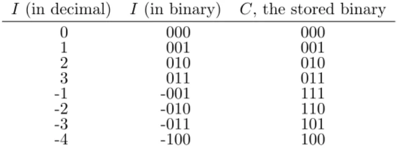
In practice the two’s-complement representation is frequently used to store signed integers. Let I be an integer which we would like to represent onm bits. Instead of I we store the binary form of the number C defined by
C =
{︃ I, if 0≤I ≤2m−1−1, 2m+I, if −2m−1 ≤I <0.
Table 1.2: Sign-magnitude binary representation onm = 3 bits I a binary code
0 000
1 001
2 010
3 011
0 100
-1 101
-2 110
-3 111
Here the largest and the smallest representable integer is Imax = 2m−1 −1 and Imin =
−2m−1, respectively. Therefore, if 0 ≤I ≤2m−1−1, thenC <2m−1, i.e., the first bit ofC is 0. On the other hand, if−2m−1 ≤I <0, then it is easy to see that 2m−1 ≤C≤2m−1, i.e., the first bit of C is 1.
An important advantage of the two’s-complement representation is that the subtrac- tion can be obtained as an addition (see Exercise 4).
Example 1.7. Table 1.3 contains all the integers which can be represented on m = 3 bits
using the two’s-complement binary representation.
□
Table 1.3: Two’s-complement representation on m= 3 bits I (in decimal) I (in binary) C, the stored binary
0 000 000
1 001 001
2 010 010
3 011 011
-1 -001 111
-2 -010 110
-3 -011 101
-4 -100 100
Next we discuss the representation of real numbers. We recall that the real number in base b number system
x= (xm−1xm−2· · ·x0.x−1x−2· · ·)b, xi ∈ {0,1, . . . , b−1}
has the numerical value
x=xm−1bm−1+xm−2bm−2+· · ·x1b+x0+ x−1
b + x−2
b2 +· · ·=
m−1
∑︂
i=−∞
xibi.
Consider the real number 126.42. Different books define the normal form of this number as 1.2642·102 or 0.12642·103. In this lecture notes we use the first form as the normal form. Therefore, the normal form of a real number x ̸= 0 in a base b number system is x=±m·bk, where 1≤m < b. The numbermis called the mantissa, andk the exponent of the number. In order to represent a real number, or in other words, afloating
1.2. Computer Representation of Integers and Reals 11 point number we write it in a normal form in a base b number system, and we would like to store its signed mantissa and exponent. Computers use different number of bits to store these numbers. Here we present an IEEE specification1 to represent floating point numbers on 32 bits (the so-called single precision), and on 64 bits (thedouble precision) using the binary number system. This representation is used in IBM PCs. Consider the binary normal form x = (−1)sm·2k, where s ∈ {0,1} and m = (1.m1m2m3. . .)2. The value s is stored in the 1st bit. Instead of the exponent k, we store its shifted value, the nonnegative integer e=k+ 127 on bits 2–9. In our definition of the binary normal form, a nonzero x has a mantissa of the form m = (1.m1m2. . .)2, i.e., it always starts with 1, which we do not store, we store the fractional digits of the mantissa rounded to 23 bits.
These 23 bits are stored on bits 10–32 of the storage. This IEEE specification defines the representation of the number 0, and introduces two special symbols,Inf(to store infinity as a possible value) and NaN(not-a-number) in the following way:
number s e (bits 2–9) mantissa bits (bits 10–32) +0 0 00000000 every mantissa bit=0
−0 1 00000000 every mantissa bit=0 +Inf 0 11111111 at least one mantissa bit=0
−Inf 1 11111111 at least one mantissa bit=0 +NaN 0 11111111 every mantissa bit=1 +NaN 1 11111111 every mantissa bit=1
The symbolInfcan be used in programs as a result of a mathematical operation with value
∞, and the symbol NaN can be a result of a mathematical operation which is undefined (e.g., a division by 0 or a root of a negative number in real numbers). Both symbols can be positive or negative. The definition yields that the exponente= (11111111)2 = 255 is used exclusively for the special symbols Inf and NaN. For finite reals the possible values are 0 ≤ e ≤ 254, hence the possible values of the exponent k are −127 ≤ k ≤ 127.
Therefore, the smallest positive representable number corresponds to exponent k=−127 and mantissa (1.00. . .01)2. Hence its value is xmin = (1 + 1/223)2−127 ≈ 10−38. The largest real can be stored is xmax = (1.11. . .1)22127 = (2−2−23)2127 ≈1038.
The representation on 64 bits is similar: the shifted exponent e =k+ 1023 is stored on bits 2–12, the fractional part of the mantissa is stored on bits 13–64. Then the range of real numbers which can be stored in the computer is, approximately, from 10−308 to 10308.
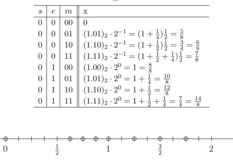
Example 1.8. Suppose we would like to store reals on 4 bits using a binary normal form. For example, we use the 1st bit as the sign bit, the shifted exponente=k+ 1 is stored on the 2nd bit, and the fractional part of the mantissa is stored on bits 3–4. (The symbols Inf and NaN are not defined now.) The nonnegative real numbers which can be represented by the above method are listed in Table 1.4, and are illustrated in Figure 1.2.
□
We can see that, using any floating point representation, we can store only finitely many reals on a computer. The reals which can be stored without an error in a certain floating point representation are called machine numbers. The machine number which is
1IEEE Binary Floating Point Arithmetic Standard, 754-1985.
Table 1.4: Nonnegative reals on 4 bits.
s e m x
0 0 00 0
0 0 01 (1.01)2·2−1= (1 + 14)12 = 58 0 0 10 (1.10)2·2−1= (1 + 12)12 = 34 = 68 0 0 11 (1.11)2·2−1= (1 + 12 +14)12 = 78 0 1 00 (1.00)2·20= 1 = 88
0 1 01 (1.01)2·20= 1 + 14 = 108 0 1 10 (1.10)2·20= 1 + 12 = 128
0 1 11 (1.11)2·20= 1 + 12+ 14 = 74 = 148
0 12 1 32 2
Figure 1.2: Nonnegative machine numbers on 4 bits.
stored in a computer instead of the real number x is denoted by fl(x). If |x| is smaller than the smallest positive machine number, then, by definition, fl(x) = 0, and if |x| is larger than the largest positive machine number, then we define fl(x) = Infforx >0 and fl(x) =−Inffor x < 0. In the first case we talk about arithmetic underflow, and in the second case, about arithmetic overflow. The definition of fl(x) in the intermediate cases can be different in different computers. There are basically two methods: In the first case we take the binary normal form of x, consider its mantissa m = (1.m1m2m3. . .)2, and we consider as many first several mantissa fractional bits as it is possible to store in the particular representation. We store them, and omit the rest of the mantissa bits.
This method is called chopping of the mantissa. For example, using the single precision representation defined above, we store the first 23 mantissa fractional bits.
The other method, the rounding, is more frequently used to define the mantissa bits of the machine number fl(x). Here the mantissa of fl(x) is defined so that fl(x) be the nearest machine number to x. In case when x is exactly an average of two consecutive machine numbers, we could round down or up. The IEEE specification for single precision representation we defined above uses the following rule: Let the normal form of a positive real x be x = m2k, where m = (1.m1m2. . . m23m24. . .)2. Let x′ = (1.m1m2. . . m23)22k and x′′=(︁
(1.m1m2. . . m23)2+ 2−23)︁
2k. Thenx′ andx′′are consecutive machine numbers, x′ ≤x≤x′′ and x′′−x′ = 2k−23. The specification defines
fl(x) =
⎧
⎪⎪
⎨
⎪⎪
⎩
x′, if |x−x′|< 12|x′′−x′|, x′′, if |x−x′′|< 12|x′′−x′|,
x′, if |x−x′|= 12|x′′−x′| and m23= 0, x′′, if |x−x′|= 12|x′′−x′| and m23= 1.
In the critical case, i.e., if |x−x′|= 12|x′′−x′|, approximately half of the cases we round down and in the other cases we round up. An other reason for this definition is that in
1.2. Computer Representation of Integers and Reals 13 this critical case the last mantissa bit is always 0, so a division by 2 can be performed on fl(x) without an error. Using the rounding, the error is
|x−fl(x)| ≤ 1
2|x′′−x′|= 1
22−232k. If we compare it to the exact value we get
|x−fl(x)|
|x| ≤ |x−fl(x)|
(1.m1m2. . .)2 ·2k ≤ 1 22−23.
We can see that the first machine number which is larger than 1 is 1 + 2−23 in the single precision floating point arithmetic. Let εm denote the difference of the first machine number right to 1 and the number 1. This number is called machine epsilon. Therefore, εm is the smallest power of 2 (in a binary storage system) for which the computer evaluates the inequality 1 +εm > 1 to be true. The following theorem can be proved similarly to the consideration above for the single precision floating point representation.
Theorem 1.9. Let 0 <fl(x) <Inf, and suppose the floating point representation uses rounding. Then
|x−fl(x)|
|x| ≤ 1 2εm. The proof of the next result is left for Exercise 5.
Theorem 1.10. Suppose we use a number system with base b, and let t be the number of mantissa bits in the floating point representation. Then
εm =
{︃ 2−t, if b = 2, b1−t, if b ̸= 2.
Now we define the notion of the error of an approximation and other related notions.
Letx be a real number, and consider ̃x as its approximation. Then the absolute error or just simply the error of the approximation is the number |x−x|. Frequently the error̃ without knowing the magnitude of the numbers does not mean too much. For example, 10000.1 can be considered as a good approximation of 10000, but in general, 1.1 is not considered as a good approximation of 1, but in both cases the errors are the same, 0.1.
We may get more information if we compare the error to the exact value. The relative error is defined by
|x−x|̃
|x| (x̸= 0).
We say that in a base b number system ̃x is exact in n digits if
|x−x|̃
|x| ≤ 1 2b1−n.
We can see that the smaller is the relative error, the larger is the number of exact digits.
In a decimal number system (b = 10) we can formulate the relation between the relative error and the number of exact digits in the following way: if the relative error decreases by a factor of 1/10, then the number of exact digits increases by 1.
Example 1.11. Letx= 1657.3 and ̃x= 1656.2. Then the absolute error is |x−x|̃ = 1.1, and the relative error is |x−x|/x̃ = 0.0006637 (with 7 decimal digits precision). Since |x−x|/x̃ = 0.0006637 < 0.5 ·10−2, the approximation is exact in 3 digits. On the other hand, if x is approximated by the value ̃x= 1656.9, then |x−x|/x̃ = 0.0002413<0.5·10−3, and hence the
approximation is exact in 4 digits.
□
The previous definition and Theorem 1.9 yield that the single precision floating point arithmetic is exact in 24 binary digits. Usually, we are interested in the exact number of digits in a decimal number system. In case of a single precision floating point arithmetic, we get it if we find the largest integer n for which
1
22−23≤ 1 2101−n.
It can be computed that n= 7 is the number of exact digits for a single precision floating point arithmetic.
Example 1.12. Consider x = 12.4. First rewrite it in binary form: 12 = (1100)2. Find the binary form of its fractional part:
0.4 = (0.x1x2x3. . .)2 = x1
2 +x2
22 +x3
23 +· · · .
If we multiply 0.4 by 2, then its integer part gives x1. 0.4·2 = 0.8, hence x1 = 0. Consider the fractional part of this product, 0.8, and we repeat the previous procedure. 0.8·2 = 1.6, so x2 = 1. The fractional part of the product is 0.6, which gives: 0.6·2 = 1.2, and therefore, x3 = 1. The fractional part of the product is 0.2. We have 0.2·2 = 0.4, hencex4 = 0, and we continue with 0.4. We can see that the digits 0011 will be repeated periodically infinitely many times, i.e., 0.4 = (0.011001100110011001100110011. . .)2. The binary normal form ofx is
x= 12.4 = (1.100011001100110011001100110011. . .)2·23. Rounding the mantissa to 23 bits (down) we get
fl(x) = (1.10001100110011001100110)2·23.
Its numerical value (in a decimal form) is fl(x) = 12.3999996185302734375.
□
The arithmetic operations performed by a computer can be defined as x⊕y:= fl(fl(x) + fl(y)),
x⊖y:= fl(fl(x)−fl(y)), x⊙y:= fl(fl(x)·fl(y)), x⊘y:= fl(fl(x)/fl(y)).
1.3. Error Analysis 15 Here we always take the machine representation of each operands and also the result of the arithmetic operation.
In later examples we will use the so-called4-digit rounding arithmetic or simply4-digit arithmetic. By this we mean a floating point arithmetic using a decimal number system with 4 stored mantissa digits (and suppose we can store any exponent). This means that, in every step of a calculation, the result is rounded to the first 4 significant digits, i.e., from the first nonzero digits for 4 digits, and this rounded number is used in the next arithmetic operation. We can enlarge the effect of rounding errors in such a way.
Example 1.13. Using a 4-digit arithmetic we get 1.043 + 32.25 = 33.29, and similarly, 1.043·32.25 = 33.64 (after rounding). But 1.043 + 20340 = 20340, since we rounded the exact
value 20341.043 to for significant digits.
□
Exercises
1. Convert the following decimal numbers to binary form:
57, −243, 0.25, 35.27 2. Convert the binary numbers to decimal form:
(101101)2, (0.10011)2, (1010.01101)2
3. Show that the two’s-complement representation of a negative integer can be computed in the following way: Take the binary form of the absolute value of the number. Change all 0’s to 1’s and all 1’s to 0’s, and add 1 to the resulting number.
4. Let I1 andI2 be two positive integers withm bits. Show that I1−I2 can be computed if we first consider the two’s-complements representation C2 of I2, add I1 to it, and finally, take the last mbits of the result.
5. Prove Theorem 1.10.
6. Write a computer code which gives back the machine epsilon of the particular computer.
7. Compute the exact number of digits of a machine number in case of a double precision floating point arithmetic.
8. Let x = (x0.x1x2. . . xmxm+1xm+2. . .)·10k, ̃x = (x0.x1x2. . . xmx̃m+1x̃m+2. . .)·10k, i.e., x and ̃x has the same order of magnitude, and its first m+ 1 digits are the same. Show that, in this case, ̃x is an approximation ofx with at leastm number of exact digits.
1.3. Error Analysis
Let x and y be positive real numbers, and consider the numbers ̃x and ̃y as an approx- imation of x and y. Let |x −x| ≤̃ ∆x and |y−y| ≤̃ ∆y be the error bounds of the approximation. The relative error bounds are denoted by δx := ∆x/x and δy := ∆y/y, respectively. In this section we examine the following question: We would like to per- form an arithmetic operation (addition, subtraction, multiplication or division) on the real numbersxandy, but instead of it, we perform the operation on the numbers ̃xand ̃y
(suppose without an error). We will consider this latter number as an “approximation” of the original one. We will examine the error and the relative error of this “approximation”.
Consider first the addition. We are looking for error bounds ∆x+y and δx+y such that
|x+y−(̃x+ ̃y)| ≤∆x+y and |x+y−(̃x+ ̃y)|
x+y ≤δx+y.
Theorem 1.14. The numbers
∆x+y := ∆x+ ∆y and δx+y := max{δx, δy} are absolute and relative error bounds of the addition, respectively.
Proof. Using the triangle inequality and the definitions of ∆x and ∆y, we get
|x+y−(̃x+ ̃y)| ≤ |x−x|̃ +|y−y| ≤̃ ∆x+ ∆y. This means that ∆x+ ∆y is an upper bound of the error of the addition.
Using the above relation, we obtain
|x+y−(̃x+ ̃y)|
x+y ≤ ∆x+ ∆y x+y
= x
x+yδx+ y x+yδy
≤max{δx, δy}.
Therefore, max{δx, δy} is a relative error bound of the addition.
□
Clearly, the above theorem can be generalized for addition of several numbers: the error bounds will be added, and the relative error bound is the maximum value of the relative error bounds. We can reformulate this result as follows: the number of exact digits of the approximation of the sum is at least the smallest of the number of exact digits of the approximations of the operands. Certainly, the theorem gives the worst case estimate. In practice the errors can balance each other. For example, let x = 1, y = 2,
̃
x = 1.1 and ̃y= 1.8. Then x+y = 3 and ̃x+ ̃y= 2.9. Therefore, the error of the sum is only 0.1, smaller than the sum of the error of the terms, 0.3.
Theorem 1.15. Let x > y >0. The numbers
∆x−y := ∆x+ ∆y and δx−y := x
x−yδx+ y x−yδy are absolute and relative error bounds of the subtraction.
Proof. The inequalities
|x−y−(̃x−y)| ≤ |x̃ −x|̃ +|y−y| ≤̃ ∆x+ ∆y
1.3. Error Analysis 17 imply the first statement. Consider
|x−y−(̃x−y)|̃
x−y ≤ ∆x+ ∆y
x−y = x
x−yδx+ y x−yδy,
which gives the second statement.
□
We can observe that if we subtract two nearly equal numbers, then the relative error can be magnified compared to the relative error of the terms. In other words, the number of exact digits can be significantly less that in the original numbers. This phenomenon is called loss of significance.
Example 1.16. Let x = 12.47531, ̃x = 12.47534, y = 12.47326 and ̃y = 12.47325. Then δx = 2.4·10−6 and δy = 8·10−7. On the other hand, x−y = 0.00205, ̃x−ỹ= 0.00209, and soδx−y = 0.0195. We can check that ̃x and ̃y are exact in 6 digits, but ̃x−ỹis exact only in 2
digits.
□
Theorem 1.17. Let x, y >0. The numbers
∆x·y :=x∆y +y∆x+ ∆x∆y, and δx·y :=δx+δy +δxδy are absolute and relative error bounds of the multiplication, respectively.
Proof. The triangle-inequality and simple algebraic manipulations yield
|xy−x̃̃y|=|xy−x̃y+x̃y−x̃y|̃
≤x|y−y|̃ +|̃y||x−x|̃
≤x∆y +|y|∆̃ x
=x∆y+|y+ ̃y−y|∆x
≤x∆y +y∆x+ ∆x∆y, hence the first statement is proved. Therefore, we get
|xy−x̃̃y|
xy ≤ x∆y+y∆x+ ∆x∆y
xy =δx+δy+δxδy,
which implies the second statement.
□
Since, in general, ∆x and ∆y are much smaller than x and y, and so ∆x∆y is much smaller than x∆y and y∆x, we have that x∆y +y∆x is a good approximation of the absolute error of the multiplication. Similarly, δx +δy is a good approximation of the relative error of the multiplication. Both results mean that the errors do not propagate rapidly in multiplication.
Theorem 1.18. Suppose x, y >0 and δy <1. Then the numbers
∆x/y := x∆y +y∆x
y(y−∆y) and δx/y := δx+δy 1−δy are absolute and relative error bounds of the division, respectively.
Proof. Elementary manipulations give
⃓
⃓
⃓
⃓ x y − x̃
̃ y
⃓
⃓
⃓
⃓
= |x̃y−xy+xy−xy|̃
y|y|̃ ≤ x∆y+y∆x
y|̃y| = x∆y+y∆x
y|y−(y−y)|̃ .
Assumption δy <1 implies|y−y| ≤̃ ∆y < y, hence|y−(y−y)| ≥̃ y− |y−y| ≥̃ y−∆y >0 proves the first statement.
For the second part, consider
⃓
⃓
⃓
x y − xỹ⃓̃
⃓
⃓
x y
= |x(̃y−y)−y(̃x−x)|
x|̃y| =
⃓
⃓
⃓
y−ỹ
y − ̃x−xx ⃓
⃓
⃓
⃓
⃓
⃓1− y−̃yy⃓
⃓
⃓
≤ δx+δy 1−δy .
□
Ifδy is small, then the relative error bound of the division can be approximated well by δx+δy. Similarly, if ∆y is much smaller thany, then 1y∆x+yx2∆y is a good approximation of ∆x/y. Ifyis much smaller thanx, or ifyis close to 0, then ∆y or ∆xcan be significantly magnified, so the absolute error can be much larger than the absolute error of the terms.
Exercises
1. Let x= 3.50,y= 10.00, ̃x= 3.47, ̃y= 10.02. Estimate the absolute and relative error of 3x+ 7y, 1
y, x2, y3, 4xy x+y
(without evaluating the expressions) assuming we replace x and y by ̃x and ̃y. Then compute the expressions numerically and compute the absolute and relative errors exactly.
Compare them with the estimates.
2. Let ̃x be an approximation of x, and |x−x| ≤̃ ∆x. Let f : R → R be a differentiable function satisfying |f′(x)| ≤M for all x∈R. Let y =f(x) and consider ̃y=f(̃x) as an approximation of y. Estimate the absolute error of the approximation. (Hint: Use the Lagrange’s Mean Value Theorem.)
1.4. The Consequences of the Floating Point Arith- metic
Example 1.19. Solve the equation
x2−83.5x+ 1.5 = 0
1.4. The Consequences of the Floating Point Arithmetic 19 using 4-digit arithmetic in the computations.
Using the quadratic formula and the 4-digit arithmetic we get the numerical values
̃
x= 83.5±√
83.52−4·1.5
2 = 83.5±√
6972−6.000
2 = 83.5±83.46
2 ,
hence
̃
x1 = 167.0
2 = 83.50, and x̃2 = 0.040
2 = 0.020.
We can check that the exact solutions (up to several digits precision) are x1 = 83.482032 and x2 = 0.0179679. Using the relative error bounds for each roots we get δ1 = 0.0002152 and δ2 = 0.113096. The first root is exact in 4 digits, but the second is only in 1 digits. So there is a significant difference between the order of the magnitudes of the relative errors. What is the reason of it? In the computation of the second root, we subtracted two close numbers. This is
the point where we significantly lost the accuracy.
□
Consider the second root of ax2+bx+c= 0:
x2 = −b−√
b2−4ac
2a . (1.2)
When b is negative and 4ac is much smaller than b2, then we subtract two nearly equal numbers, and we observe the loss of significance. (This happened for the second root in Example 1.19.) To avoid this problem, consider
x2 = b2−(b2−4ac) 2a(−b+√
b2−4ac) = 2c
−b+√
b2−4ac. (1.3)
This formula is algebraically equivalent to formula (1.2). But the difference is that here we do not subtract two close numbers (in the denominator we add two positive numbers).
If b is positive, then for the first root we get
x1 = 2c
−b−√
b2−4ac. (1.4)
Example 1.20. Compute the second root of the equation of Example 1.20 using 4-digit arithmetic and formula (1.3).
̃
x2 = 2·1.5 83.5 +√
83.52−4·1.5 = 3
83.5 + 83.46 = 3
167.0 = 0.01796.
The relative error of x2 is nowδ2 = 0.00044, hence the exact number of digits is 4.
□
Example 1.21. Suppose we need to evaluate the expression cos2x−sin2x. Ifx= π4, then the exact value of this expression is 0, hence if x is close to π4, then in the expression we need to subtract to nearly equal numbers, so we can face loss of significance. We can avoid it if, instead of the original formula, we evaluate its equivalent form, cos 2x.
□
In the previous examples we used algebraic manipulations to avoid the loss of signifi- cance. Now we show different techniques.
Example 1.22. Consider the function f(x) =ex−1. In the neighborhood of x= 0 we again need to subtract two nearly equal numbers, but here we cannot use an algebraic identity to avoid it. But here we can consider the Taylor series of the exponential function, and we get
f(x) =x+x 2 + x3
3! +· · ·+xn
n! +· · · .
It is worth to take a finite approximation of this infinite series, and use it as an approximation
of the function value f(x).
□
The next example shows a different problem.
Example 1.23. Evaluate the number y = 2050/50!. The problem is the following: If we compute the numerator and the denominator separately first, then we run into the problem of overflowing the calculation if we use single precision floating point arithmetic. On the other hand, we know that an/n!→0 asn→ ∞, so the result must be a small number. We rearrange the computation as follows:
2050 50! = 20
50 ·20 49·20
48· · ·20 1 .
Here in each steps the expressions we need to evaluate belong to the range which can be stored in the computer. This formula can be computed with a simple for cycle:
y ←20
for i= 2, . . . ,50do y←y·20i end do
output(y)
The result is 3.701902 (with 7-digits precision).
□
Example 1.24. Compute the sum
A= 10.00 + 0.002 + 0.002 +· · ·+ 0.002 = 10.00 +
10
∑︂
i=1
0.002
using a 4-digit arithmetic. We perform the additions from left to right, so first we need to compute 10.00 + 0.002. But with a 4-digit arithmetic the result is 10.00 + 0.002 = 10.002 = 10.00 after the rounding. Adding the next number to it, because of the rounding to 4 digits, we get again 10.00 + 0.002 + 0.002 = 10.00. Hence we get the numerical resultA= 10.00.
Consider the same sum, but in another order:
B = 0.002 + 0.002 +· · ·+ 0.002 + 10.00 =
10
∑︂
i=1
0.002 + 10.00.
First we need to compute 0.002 + 0.002 = 0.004. The result is exact even if we use 4-digit arithmetic. Then we can continue: 0.002 + 0.002 + 0.002 = 0.006 etc., and finally, ∑︁10
i=10.002 =
1.4. The Consequences of the Floating Point Arithmetic 21 0.02. Therefore, the numerical result will beB = 10.02. Here we have not observed any rounding error, since we could compute the result in each step exactly.
This example demonstrates that the addition using a floating point arithmetic is not a
commutative operation numerically.
□
A conclusion of the previous example is that in computing sums with several terms, it is advantageous to do the computation in an increasing order of the terms, since in that case we have a better chance for that the terms have similar order of magnitude, so the loss of significance has less chance.
Exercises
1. Investigate that in the next example what are the cases when we can observe the loss of significance. How can we avoid it?
(a) lnx−1, (b) √
x+ 4−2, (c) sinx−x, (d) 1−cosx,
(e) (1−cosx)/sinx, (f) (cosx−e−x)/x,
2. Compute the next expression using a 4-digit arithmetic 2.274 + 12.04 + 0.4233 + 0.1202 + 0.2204, and then sort the terms in an increasing way, and repeat the calculation.
Chapter 2
Nonlinear Algebraic Equations and Systems
In this chapter we investigate numerical solution of scalar nonlinear algebraic equations and systems of nonlinear algebraic equations. We discuss the methods of bisection, false position, secant, Newton and quasi-Newton. We introduce the basic theory of fixed points, the notion of the speed of convergence, stopping criteria of iteration methods. We define the notion of vector and matrix norms, and discuss convergence of vector sequences.
2.1. Review of Calculus
In this section we summarize some basic results and notions from Calculus which will be needed in our later sections.
C[a, b] will denote the set of continuous real valued functions defined on the interval [a, b]. Cm[a, b] will denote the set of continuous real valued functionsf: [a, b]→R, which are m-times continuously differentiable on the open interval (a, b).
Theorem 2.1. Let f ∈C[a, b]. Then f has its maximum and minimum on the interval [a, b], i.e., there exist c, d∈[a, b], such that
f(c) = max
x∈[a,b]f(x) and f(d) = min
x∈[a,b]f(x).
The open interval spanned by the numbers a and b is denoted by ⟨a, b⟩, i.e., ⟨a, b⟩:=
(min{a, b},max{a, b}). In general, ⟨a1, a2, . . . , an⟩ denotes the open interval spanned by the numbers a1, a2, . . ., an, i.e.,
⟨a1, a2, . . . , an⟩:= (min{a1, a2, . . . , an},max{a1, a2, . . . , an}).
The next result, the so-called Intermediate Value Theorem, states that a continuous function takes any value in between two function values.
Theorem 2.2 (Intermediate Value Theorem). Let f ∈C[a, b], f(a)̸=f(b), and let d∈ ⟨f(a), f(b)⟩. Then there exists c∈(a, b) such that f(c) =d.
Theorem 2.3 (Rolle’s Theorem). Let f ∈C1[a, b] andf(a) = f(b). Then there exists ξ ∈(a, b) such that f′(ξ) = 0.
Theorem 2.4 (Lagrange’s Mean Value Theorem). Let f ∈ C1[a, b]. Then there exists ξ ∈(a, b) such that f(b)−f(a) = f′(ξ)(b−a).
Theorem 2.5 (Taylor’s Theorem). Let f ∈ Cn+1[a, b], and let x0 ∈ (a, b). Then for every x∈(a, b) there exists ξ=ξ(x)∈ ⟨x, x0⟩ such that
f(x) = f(x0) +f′(x0)(x−x0) + f′′(x0)
2 (x−x0)2+· · ·+ f(n)(x0)
n! (x−x0)n + f(n+1)(ξ)
(n+ 1)! (x−x0)n+1.
The next result is called the Mean Value Theorem for integrals.
Theorem 2.6. Let f ∈C[a, b], g: [a, b]→R is integrable which has no sign change on [a, b] (i.e., g(x)≥0 or g(x)≤0 holds for all x∈[a, b]). Then there exists ξ ∈(a, b) such that
∫︂ b a
f(x)g(x)dx=f(ξ)
∫︂ b a
g(x)dx.
The next result is called Cantor’s Intersection Theorem.
Theorem 2.7. Let [an, bn] (n= 1,2, . . .) be a sequence of closed and bounded intervals, for which [an+1, bn+1]⊂[an, bn] holds for all n and (bn−an)→0 as n → ∞. Then there exists a c∈[a1, b1] such that an→c and bn→c as n → ∞.
Theorem 2.8. A monotone and bounded real sequence has a finite limit.
We close this section with a result from algebra, which we state in the following form.
Theorem 2.9 (Fundamental Theorem of Algebra). Any nth-degree polynomial p(x) =anxn+· · ·a1x+a0, aj ∈C (j = 0, . . . , n), an ̸= 0
has exactly n complex roots with counting multiplicities.
We will use the following consequence of the previous result. If a polynomial of the form p(x) = anxn+· · ·+a1x+a0 has n+ 1 different roots, then p(x) = 0 for all x∈R.
2.2. Fixed-Point Iteration
Many numerical methods generate an infinite sequence whose limit gives the exact solution of the investigated problem. The sequence is frequently defined by arecursionoriteration.
A recursion of the form pk+1 = h(pk, pk−1, . . . , pk−m+1) (k ≥ m−1) is called m-order
2.2. Fixed-Point Iteration 25 recursion or m-step iteration. An m-step iteration is well-defined if m number of initial values p0, p1, . . ., pm−1 are given.
In this section we study the one-step iteration, the so-calledfixed-point iteration. Given a function g: I → R, where I ⊂ R. The recursive sequence pk+1 = g(pk) which corre- sponds to an initial value p0 ∈I is called a fixed-point iteration.
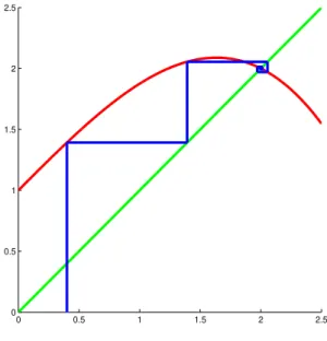
Example 2.10. Consider the function g(x) =−18x3+x+ 1. In Table 2.1 we computed the first few terms of the fixed-point iteration starting from the value p0 = 0.4. We illustrate the sequence in Figure 2.1. Such picture is called stair step diagram orCobweb diagram. From the starting point (p0,0) we draw a vertical line segment to the graph ofg. The second coordinate of the intersection gives p1. From the point (p0, p1) we draw a horizontal line segment to the point (p1, p1) on the line y =x. Now we get the valuep2 = g(p1) as the second coordinate of the intersection of the vertical line starting from this point and the graph ofg. Continuing this procedure we get the figure displayed in Figure 2.1. The line segments spiral and get closer and closer to the intersection of the graphs of the line y=x and the function g. The coordinates of the intersection is (2,2). From Table 2.1 it can be seen that the sequence pk converges to 2.
□
Table 2.1: Fixed-point iteration, g(x) =−18x3+x+ 1
k pk
0 0.40000000 1 1.39200000 2 2.05484646 3 1.97030004 4 2.01419169 5 1.99275275 6 2.00358428 7 1.99819822 8 2.00089846 9 1.99955017 10 2.00022477 11 1.99988758 12 2.00005620 13 1.99997190 14 2.00001405 15 1.99999297
In the previous example we observed that the fixed-point iteration converged to the first coordinate of the intersection of the graphs of the line y = x and the function y = g(x). The first (and also the second) coordinate of this point satisfies the equation g(x) =x. The number p is called thefixed point of the function g if it satisfies
g(p) = p.
Using this terminology in the previous example the fixed-point iteration converged to the fixed point of the function g. The next result shows that this is true for all convergent fixed-point iterations if the function g is continuous.
Theorem 2.11. Letg: [a, b]→[a, b](orR→R) be a continuous function,p0 ∈[a, b]be fixed, and consider the fixed-point iteration pk+1 =g(pk). If pk is convergent and pk→p, then p=g(p).
Proof. Since pk+1 =g(pk) and pk+1 →p by the assumptions, the continuity of g yields
g(pk)→g(p) as k → ∞, hence the statement follows.
□
0 0.5 1 1.5 2 2.5 0
0.5 1 1.5 2 2.5
Figure 2.1: Fixed-point iteration
A fixed-point iteration is not always convergent, or the limit is not necessary finite.
To see that it is enough to consider the function g(x) = 2x and the initial value p0 = 1.
Then pk = 2k, and it converges to infinity. And if we consider g(x) = −x and p0 = 1, then the corresponding fixed-point sequence is pk = (−1)k, which is not convergent.
The next theorem gives sufficient conditions for the existence and uniqueness of the fixed point.
Theorem 2.12. Let g : [a, b] → [a, b] be continuous. Then g has a fixed point in the interval [a, b]. Moreover, if g is differentiable on (a, b), and there exists a constant 0≤c <1 such that |g′(x)| ≤c for all x∈(a, b), then this fixed point is unique.
Proof. Consider the functionf(x) =g(x)−x. If f(a) = 0 or f(b) = 0, then a or b is a fixed point of g. Otherwise,f(a)>0 and f(b)<0. But then the continuity off and the Intermediate Value Theorem imply that there exists a p∈(a, b), such thatf(p) = 0, i.e., p=g(p).
For the proof of the uniqueness, suppose thatg has two fixed points pand q. Then it follows from the Lagrange’s Mean Value Theorem that there exists a ξ∈(a, b) such that
|p−q|=|g(p)−g(q)|=|g′(ξ)||p−q| ≤c|p−q|.
But this yields that p=q, i.e., the fixed point is unique.
□
Theorem 2.13 (fixed-point theorem). Let g: [a, b]→[a, b] be continuous,g is differ- entiable on (a, b), and suppose that there exists a constant 0≤c < 1such that |g′(x)| ≤c for all x ∈(a, b). Let p0 ∈ [a, b] arbitrary, and pk+1 =g(pk) (k ≥ 0). Then the sequence pk converges to the unique fixed point p of the function g,
|pk−p| ≤ck|p0−p|, (2.1)
2.2. Fixed-Point Iteration 27 and
|pk−p| ≤ ck
1−c|p1−p0|. (2.2)
Proof. Theorem 2.12 implies that g has a unique fixed pointp. Since 0 ≤c <1 by our assumptions, the convergencepk →pfollows from (2.1). To show (2.1), we have from the assumptions and the Lagrange’s Mean Value Theorem that
|pk−p|=|g(pk−1)−g(p)|=|g′(ξ)||pk−1−p| ≤c|pk−1−p|.
Now mathematical induction gives relation (2.1) easily.
To prove (2.2), let m > k be arbitrary. Then the triangle inequality, the Mean Value Theorem and our assumptions imply
|pk−pm| ≤ |pk−pk+1|+|pk+1−pk+2|+· · ·+|pm−1−pm|
≤ |g(pk−1)−g(pk)|+|g(pk)−g(pk+1)|+· · ·+|g(pm−2)−g(pm−1)|
≤c|pk−1−pk|+c|pk−pk+1|+· · ·+c|pm−2−pm−1|
≤(ck+ck+1+· · ·+cm−1)|p0−p1|
=ck(1 +c+· · ·+cm−k−1)|p1−p0|
≤ck
∞
∑︂
i=0
ci|p1−p0|.
Hence |pk−pm| ≤ 1−cck |p1−p0| holds for allm > k. Keeping k fixed and tending with m
to∞, we get (2.2).
□
We remark that in the proof of the previous two theorems, the differentiability of g and the boundedness of the derivative is used only to get the estimate
|g(x)−g(y)| ≤c|x−y|. (2.3) We say that the function g: I →Ris Lipschitz continuous on the interval I, or in other words, it has the Lipschitz property if there exists a constant c≥0 such that (2.3) holds for all x, y ∈I. The constant cin (2.3) is called the Lipschitz constant of the function g.
Clearly, if g is Lipschitz continuous on I, then it is also continuous on I. From the Lagrange’s Mean Value Theorem we get that ifg ∈C1[a, b], theng is Lipschitz continuous on [a, b] with the Lipschitz constant c := max{|g′(x)|: x ∈ [a, b]}. g is also Lipschitz continuous if it is only piecewise continuously differentiable. One example is the function g(x) = |x|. If g is Lipschitz continuous with a Lipschitz constant 0 ≤ c < 1, then g is called acontraction. Theorem 2.13 can be stated in the following more general form.
Theorem 2.14 (contraction principle).Let the function g: [a, b]→[a, b]be a contrac- tion, p0 ∈ [a, b] be arbitrary, and pk+1 = g(pk) (k ≥ 0). Then the sequence pk converges to the unique fixed point p of the functiong, and relations (2.1) and (2.2) are satisfied.
In numerics we frequently encounter with iterative methods which converge assuming the initial value is close enough to the exact solution of the problem, i.e., to the limit
of the sequence. We introduce the following notion. We say that the iteration pk+1 = h(pk, pk−1, . . . , pk−m+1)converges locally topif there exists a constantδ >0, such that for every initial valuep0, p1, . . . , pm−1 ∈(p−δ, p+δ) the corresponding sequencepk converges to p. If the iteration pk converges to p for every initial value, then this iteration method is called globally convergent.
Theorem 2.15. Let g ∈ C1[a, b], and let p ∈ (a, b) be a fixed point of g. Suppose also that |g′(p)| < 1. Then the fixed-point iteration converges locally to p, i.e., there exists a δ > 0 such that pk+1 =g(pk) converges to p for all p0 ∈(p−δ, p+δ).
Proof. Sinceg′ is continuous and|g′(p)|<1, there exists aδ > 0 such that [p−δ, p+δ]⊂ (a, b) and|g′(x)|<1 for x∈[p−δ, p+δ]. Letc:= max{|g′(x)|: x∈[p−δ, p+δ]}. Then 0≤c <1.
We show thatg maps the interval [p−δ, p+δ] into itself. Let p0 ∈[p−δ, p+δ]. The Lagrange’s Mean Value Theorem and the definition of c yield
|g(p0)−p|=|g(p0)−g(p)| ≤c|p0−p|<|p0 −p|< δ,
i.e., g(p0) ∈ [p−δ, p +δ]. Therefore, Theorem 2.13 can be applied for the function g restricting it to the interval [p−δ, p+δ], which proves the result.
□
Exercises
1. Let g(x) = mx, where m ∈ R. Draw the stair step diagram of the fixed-point it- eration corresponding to g and to any non-zero initial value for the parameter values m= 0.5,1,1.5,−0.5,−1,−1.5.
2. Rewrite the following equation as a fixed-point equation, and approximate its solution by a fixed-point iteration with a 4-digit accuracy.
(a) (x−2)3=x+ 1, (b) cosxx = 2,
(c) x3+x−1 = 0, (d) 2xsinx= 4−3x.
3. Consider the equation x3+x2+ 3x−5 = 0. Show that the left hand side is monotone increasing, and has a root on the interval [0,2]. (It is easy to see that the exact root is x= 1.) Verify that the equation is equivalent to all of the following fixed-point problems.
(a) x=x3+x2+ 4x−5, (b) x=√3
5−x2−3x, (c) x= x2+x+35 , (d) x= 5−xx+33,
(e) x= 2x3x32+x+2x+32+5, (f) x= 5+7x−x102−x3.
Compute the first several terms of the associated fixed-point iteration using the starting value p0 = 0.5, and determine if we get a convergent sequence from this starting value.
Compare the speed of the convergence of the sequences.
4. Prove that the recursionpk = 12pk−1+p1
k−1 converges to√
2, if p0>√
2. What do we get if 0< p0<√
2, or ifp0<0?
5. Prove that the sequencepk= 12pk−1+2pA
k−1 converges to√
A, if p0 >0. What happens if p0<0?
![Table 2.2: bisection method, f(x) = e x − 2 cos x, [0, 1], ε = 10 −5](https://thumb-eu.123doks.com/thumbv2/9dokorg/1138843.81226/30.918.207.677.253.548/table-bisection-method-f-x-e-cos-ε.webp)
![Table 2.3: Method of false position, f (x) = e x − 2 cos x, [0, 1], T OL = 10 −5](https://thumb-eu.123doks.com/thumbv2/9dokorg/1138843.81226/32.918.206.704.613.786/table-method-false-position-f-cos-t-ol.webp)