´Obuda University

(1)

Obuda University ´

PhD thesis

Controller-managed automated therapy and tumor growth model identification in the case of antiangiogenic therapy for most effective, individualized treatment

by

Johanna S´ ajevicsn´e S´ api Supervisor:

Levente Adalbert Kov´ acs PhD, habil.

Doctoral School of Applied Informatics and

Applied Mathematics

(2)

First and foremost, I would like to express my special appreciation to my supervisor, Dr. Levente Kov´acs. Without his assistance and useful advice in every step throughout my studies, this dissertation would have never been accomplished. He is a great leader, researcher – and let me say – friend.

I would like to thank my teachers, from whom I learnt a lot. During my Bachelor’s studies at Semmelweis University Dr. András Jávor,Dr. Péter Csépe andZoltán Sára launched me on my way to medical and informatics sciences. I have to thank Prof.

Zoltán Benyó who is one of the founders of biomedical engineering in Hungary; his persistent work provided me the possibility of my Master’s studies at Budapest University of Technology and Economics. Dr. Katalin Friedl andProf. Béla Lantoswere exemplary to me during my PhD studies at Budapest University of Technology and Economics with their knowledge and modesty.

I would also like to thank Rector Prof. Imre J. Rudas and the leaders of the Doctoral School of Applied Informatics and Applied Mathematics at Óbuda University,Prof. Aurél Galántai and Prof. László Horváth for their support.

I have to thank my colleagues with whom I have worked together in the current research topic,Dániel András Drexler,Dr. István Harmati and Annamária Szeles.

I express my warm thanks to my parents, who supported me during my studies;

especially to my father, who have lead me throughout my academic journey.

I would like to say special thanks to my husband, who encouraged me throughout my research. Without his heartening and sincere love, none of this work would have happened.

I would like to say special thanks tomy twin sister. She taught me in the bathroom of the primary school when we were approximately 9 years-old how to write big numbers correctly. In addition she has always helped and supported me during my whole life.

Also, I want to say thanks to all my family members: my grandmothers, my grandfather, my sisters andmy brothers-in-law. I am very grateful having such a big and lovely family.

This thesis stands as a testament to God’s unconditional love. Soli Deo Gloria!

(5)

List of Figures

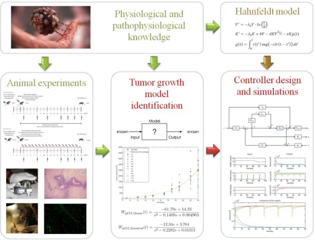
1.1 Concept of my research. Tumor growth dynamics under angiogenic inhibition is described by Hahnfeldt model. I have investigated the model, designed controllers and made simulations. In the light of new medical researches, it has become clear that there is a strong need to revise this tumor growth model. Animal experiments were done to create a new model. 2 2.1 FDA approved monoclonal antibodies (mAbs) for cancer therapy (Becker

2011). . . 7 2.2 Angiogenesis in cancer development, growth, and metastasis (Hoeben et al.

2004). . . 9 3.1 Tumor growth without angiogenic therapy (upper figure) and under con-

stant angiogenic inhibition (lower figure) . . . 17 4.1 The equilibrium point of the closed-loop system. The equilibrium y^∗ is

the intersection of the curve d/e y^2/3 (solid) and the line (k₁+k₂)y+b/e (dashdot). The rate of change of the vasculature volume is the difference of the line and the curve. . . 26 4.2 Design structure for linear state-feedback control. In the case of pole

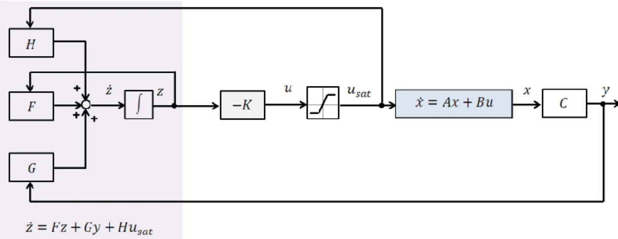
placement, the feedback matrix K is calculated by using the Ackermann’s formula; in the case of LQ optimal control, K is calculated from the solution of the CARE equation. Since linear controller strategies may result in high valued control signal, saturation was applied for the control signal in light of physiological aspects. . . 29 4.3 Design stucture for linear state-feedback with observer. Since linear

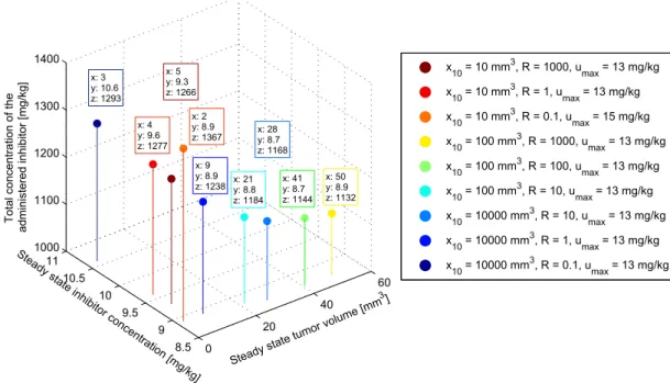
controller strategies may result in high valued control signal, saturation was applied for the control signal in light of physiological aspects. . . 30 4.4 Visualization of suboptimal controls which have near-optimal values for

both criteria. Axes are the evaluated three criteria. . . 38

(6)

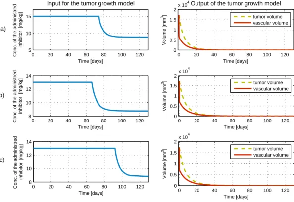
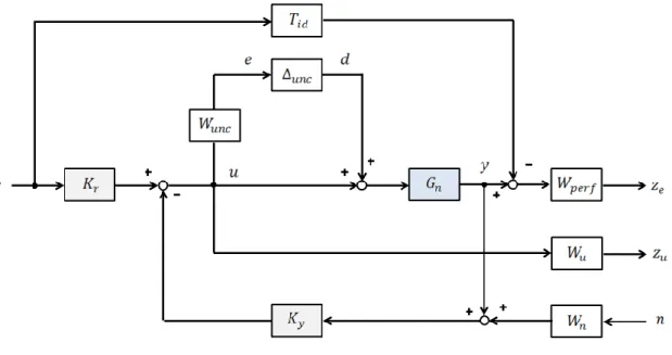
4.5 Input and output signals of the tumor growth model in the case of suboptimal contol parameters. a) Controller: LQ control method, x₁₀= 10 mm³, R = 0.1, umax = 15 mg/kg. Period of maximum inhibitor dosage is 74 days, achieving the steady state inhibitor dosage in 101 days, achieving the steady state tumor volume in 73 days. b) Controller: LQ control method, x10= 100 mm³, R= 10,umax= 13 mg/kg. Period of maximum inhibitor dosage is 66 days, achieving the steady state inhibitor dosage in 97 days, achieving the steady state tumor volume in 67 days. c) Controller: LQ control method, x10= 10000 mm³,R= 0.1,umax = 13 mg/kg. Period of maximum inhibitor dosage is 92 days, achieving the steady state inhibitor dosage in 121 days, achieving the steady state tumor volume in 89 days. . 39 4.6 The closed-loop interconnection structure forH∞ controller design . . . . 42 4.7 The generalized ∆−P−K structure . . . 43 4.8 Weighting functions of the controller . . . 47 4.9 Robust Performance, Robust Stability and Nominal Performance . . . 48 4.10 Investigating the effect of different operating points on the a) steady

state tumor volume, b) steady state inhibitor concentration, c) period of maximal inhibitor dose and d) total concentration of the administered inhibitor . . . 50 4.11 Comparison of control inputs and tumor volumes in the cases of Linear

Quadratic optimal control and suboptimal Robust Control method . . . . 51 4.12 Comparison of changes in tumor volume after making the diagnosis (14137

mm³) in three different cases: a) therapy using the controller which was designed with Robust Control method b) therapy based on the Hungarian OEP protocol for antiangiogenic monotherapy c) without therapy . . . 52 4.13 Relative modeling error functions (perturbed system compared to the

nominal model) in frequency domain and uncertainty upper bound (dashed line). . . 54 4.14 Characteristics of tumor regression and control input in case of different

perturbation scenarios – parameters change between the 5th and 10th day (blue), the 10th and 15th day (red) and the 15th and 20th day (green), each model parameter is perturbed independently with a variability of

±25%. . . 55

(7)

4.15 The total inhibitor inlet in case of different perturbation scenarios – parameters change between the 5th and 10th day (blue), the 10th and 15th day (red) and the 15th and 20th day (green), each model parameter is perturbed independently with a variability of±25%. . . 57 5.1 In Phase I, tumor growth was investigated without antiangiogenic therapy

with two types of mouse tumor (C38 colon adenocarcinoma and B16 melanoma). Mice were sacrificed when the tumor reached a lethal size (in the case of B16 melanoma it was the 16th day of the experiment, in the case of C38 colon adenocarcinoma it was the 24th day). Tumor volume was measured with digital caliper. . . 61 5.2 In Phase II, the toxicology investigation of the applied angiogenic inhibitor

was performed. There was no serious toxic side-effect or lethality regarding to the usage of bevacizumab. . . 62 5.3 In Phase III/1, C38 colon adenocarcinoma growth was investigated with

bevacizumab therapy. Control group received 10 mg per kg body weight bevacizumab, while case group received one-tenth dose of control dose spread over 18 days. Bevacizumab administration was started on the 7th day in both cases. Quantity of the optimal solvent administration was also examined in this subphase. Tumor volume was measured with digital caliper.. . . 63 5.4 In Phase III/2, C38 colon adenocarcinoma growth was investigated with

bevacizumab therapy. Control group received 10 mg per kg body weight bevacizumab, while case group received one-tenth dose of control dose spread over 18 days. Bevacizumab administration was started on the 3rd day in both cases. Tumor volume was measured with digital caliper. . . . 64 5.5 In Phase III/3, C38 colon adenocarcinoma growth was investigated with

bevacizumab therapy. Control group received 10 mg per kg body weight dose for an 18-day therapy (on the 3rd and 21st days), while case group received one-tenth dose of control dose spread over 18 days (every day for 20 days). Bevacizumab administration was started on the 3rd day in both cases. Tumor volume was measured with digital caliper and by small animal MRI. . . 65 5.6 Measuring two diameters (width, length) of the tumor with digital caliper. 69 5.7 MRI slices in the case of a control group mouse (C4) on the 23rd day of

the experiment (Phase III/3). . . 70

(8)

5.8 Stained slices in the case ofn1 mouse (Phase I, 24th day of the experiment).

a) Haematoxylin Eosin (H&E) staining was applied to investigate tumor morphology. b) Fluorescence picture was created using CD31 antibody immunohistochemistry staining to calculate vascularization area. . . 73 6.1 Exponential curve fitting for average in the case of C38 colon adenocarci-

noma (y(t) =−0.076·exp(0.4239t) + 16.87·exp(0.2329t) . . . 77 6.2 Linear regression between tumor mass and volume in the case of C38 colon

adenocarcinoma (R²= 0.871, R= 0.933, p <0.0001) . . . 79 6.3 Linear regression between tumor mass and vascularization in the case of

C38 colon adenocarcinoma (R² = 0.039, R= 0.198, p= 0.584) . . . 79 6.4 Linear regression between tumor volume and vascularization in the case

of C38 colon adenocarcinoma (R²= 0.069, R= 0.263, p= 0.462) . . . 79 6.5 Exponential curve fitting for average in the case of B16 melanoma (y(t) =

−511.6·exp(0.54781t) + 512.3·exp(0.54775t) . . . 81 6.6 Linear regression between tumor mass and volume in the case of B16

melanoma (R² = 0.421, R= 0.649, p= 0.042) . . . 82 6.7 Linear regression between tumor mass and vascularization in the case of

B16 melanoma (R²= 0.215, R= 0.463, p= 0.177). . . 82 6.8 Linear regression between tumor volume and vascularization in the case

of B16 melanoma (R² = 0.029, R= 0.170, p= 0.638) . . . 82 6.9 Comparison of C38 colon adenocarcinoma growth in three different cases.

In Phase I, tumor growth was investigated without antiangiogenic therapy;

in Phase III/2, control group members received one 200 µg bevacizumab dose for a 18-day therapy; in Phase III/2, case group members received 1.11µg bevacizumab every day for 18 days. The first row shows the second order exponential curve fitting for the average of measurement points; in the second row one can see the impulse response of the identified systems;

while the third row shows the poles and zeros of the identified systems. . 84

(9)

6.10 Linear regression analysis for tumor volume – tumor mass, tumor volume – vascularization, and tumor mass – vascularization pairs. In Phase I, tumor growth was investigated without antiangiogenic therapy; in Phase III/2, control group members received one 200µg bevacizumab dose for a 18-day therapy; in Phase III/2, case group members received 1.11µg bevacizumab every day for 18 days. R is the Pearson correlation coefficient, R² is the coefficient of determination,p is the ANOVA significance value (level of significance is p= 0.05). . . 86 6.11 Validation of caliper-measured data. The figure shows the results of a

mouse (C4) from control group (first row), and a mouse (E9) from case group (second row). The first column shows the tumor values which were calculated using the two-dimensional mathematical model; the second column represents the protocol-based tumor volumes. In each case the reference value is the MRI-measured tumor volume. One can see that the two-dimensional mathematical model fits to the MRI-measured values, while the protocol-based values present totally different curve.. . . 89 6.12 Evaluation of Phase I tumor volume values. ”Measured data” is the MRI-

measured tumor volume – tumor mass pairs on the 23rd day of Phase III/3 (case and control group). For this dataset, linear curve fitting was carried out (”fitted linear curve”) to find the mathematical relationship between MRI-measured tumor volume and tumor mass. Substituting tumor mass values – which were measured on the 24th day of Phase I – to the equation of the resulted curve, the corresponding tumor volume values can be evaluated (”evaluated data”). . . 92 6.13 Illustration for tumor with irregular structure (berry-shaped). a) berry-

shaped tumor; b)x-diameter of the tumor; c) y-diameter of the tumor; d) z-diameter of the tumor; e) berry-shaped tumor with ellipsoidal estimation.

Even though all the three diameters can be measured, the estimation of the volume has quite a large error. . . 93 6.14 Average of tumor volumes for every measurement days of the experiment

in the case of Phase I, Phase III/3 control and Phase III/3 case group.

The significant difference between quasi-continuous therapy (Phase III/3 case group) and tumor growth without treatment (Phase I) was proved with statistical analysis as well. . . 94

(10)

List of Tables

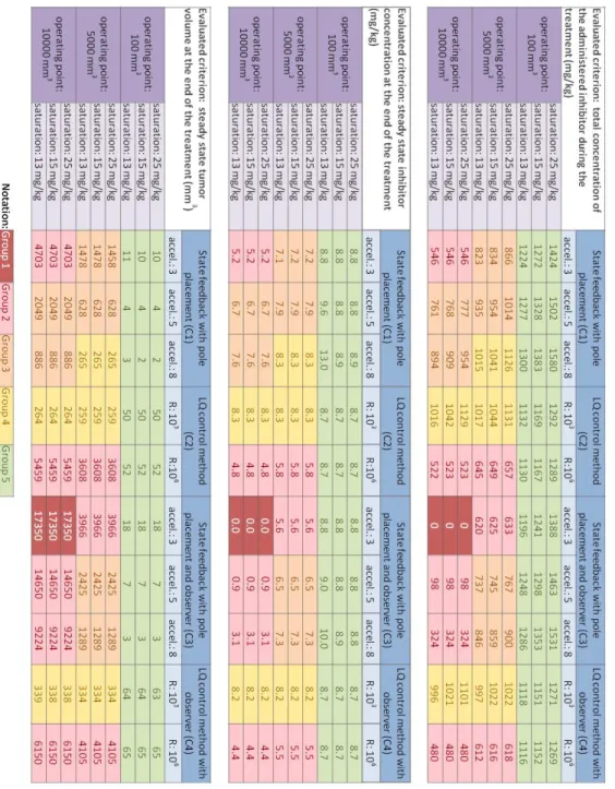
3.1 Parameters of the original model of Hahnfeldt et al. 1999 . . . 13 4.1 Simulation results for all of the investigated controller types. Notation:

Group 1: tumor volume was not reduced; Group 2: high steady state tumor volume;Group 3: medium steady state tumor volume;Group 4: low steady state tumor volume; Group 5: nearly avascular steady state tumor volume, successful control. Simulation period was 100 days. . . 34 4.2 Simulation results for LQ control method in the extended range ofR, with

a new operating point. Suboptimal controls for both criteria are marked.

Simulation period was 100 days. . . 37 5.1 Experimental settings for small animal MRI measurement in Phase III/3. 72 6.1 Experimental data (tumor length, tumor width, tumor mass and tumor

volume). . . 91

(11)

Abstract

Examination of tumor growth and optimal administration of anticancer drugs belongs not only to basic medical research, but to the fields of biomedical engineering and applied informatics as well. The aim of physiological modeling and control is to study, understand and model biological processes, then to apply identification and control strategies upon it.

By designing closed-loop control systems, the empirically determined and constant drug dosage prescribing medical protocols could become model-based. Model-based design enables the automated treatment of cancer diseases by the personalized administration of antiangiogenic (new blood vessel creation inhibitor) drugs. In this way, more effective remedial solutions can be found and individualized treatment for the patient.

This approach is a completely novel one and may lead to a breakthrough in cancer therapies. Optimizing cancer treatments would improve efficiency, decrease treatment cost and minimize the side effects of cancer therapy (i.e. improves the patient’s quality of life); thus analysis and synthesis of cancer therapies from an engineering point of view is needed.

The dissertation contains two main thesis groups. The first thesis group provides linear control synthesis for antiangiogenic therapy over the simplified tumor growth model of Hahnfeldt et al. 1999. Two different control methods were applied to design linear controllers. Linear state-feedback control was carried out with pole placement and LQ optimal control as well. Since not every state variables of the system can be measured, a linear observer was designed for both state-feedback methods. I investigated several parameter changes to observe the effect of the different control parameters: four operating points, three pole acceleration values (in the case of pole placement) and three saturation limits were analyzed; in addition, R weighting matrix (in the case of LQ optimal control) was examined over a wide range of values. Every simulation result was evaluated based on three criteria which are relevant from the medical and engineering points of view.

The other applied method is robust (H∞) control. Taking into account the fact that every model contains uncertainties and measurement noises, there is a need for systems which satisfy the requirements not only for its nominal values but also in the presence of perturbations. I designed a stabilizing robust controller, where ideal system and weighting functions were chosen in the light of physiological aspects. The results of Robust control were compared to the results based on LQ optimal control and the Hungarian OEP

(12)

The second thesis group provides tumor growth model identification. Specific animal experiments were performed to investigate tumor growth dynamics and create new tumor growth models. Tumor growth was investigated without therapy and under angiogenic inhibition. Linear model identification of tumor growth dynamics without therapy using parametric identification was carried out on two tumor types (C38 colon adenocarcinoma and B16 melanoma). Linear model identification of C38 colon adenocarcinoma growth dynamics under bevacizumab inhibition was performed using parametric identification as well. The resulting models are clinically valid and sufficiently simple to be manageable for both real-life applicability and controller design.

The relationship between the measured tumor attributes during the experiments (tumor mass, tumor volume and vascularization) was examined using linear regression analysis.

Tumor volumes were calculated using caliper-measured data and small animal MRI measurement results. A two-dimensional mathematical model was created for tumor volume evaluation from caliper-measured data; it resulting in more precise tumor volume evaluation than the Xenograft Tumor Model Protocol. Effective dosage of angiogenic inhibitor for optimal cancer therapy was also investigated, and quasi-continuous therapy was found to be more effective than protocol-based therapy.

(13)

Absztrakt

A tumornövekedés és az optimális daganatellenes szerek adagolásának vizsgálata nem csupán az orvostudomány kutatási területéhez tartozik, hanem az orvosbiológiai/egészség-

¨

ugyi mérnöki és az alkalmazott informatikai kutatási területekhez is. Az élettani folyama- tok modellezésének és szabályozásának célja, hogy tanulmányozza, megértse és modellezze az egyes biológiai folyamatokat, majd identifikációs és szabályozótervezési módszertant alkalmazzon a feláll´ıtott modellre. Zárt hurkú szabályozások tervezésével az empirikusan meghatározott és konstans gyógyszeradagolást el˝o´ıró orvosi protokollok modell-alapúvá válhatnak. A modell-alapú tervezés lehet˝ové teszi a daganatos betegségek automatizált kezelését az antiangiogén (új ér képz˝odését gátló) gyógyszerek egyéni adagolásával. Ezáltal még hatékonyabb megoldások találhatók a gyógy´ıtásban és a beteg személyre szabott kezelésben részes´ıthet˝o.

Ez a megközel´ıtés teljesen új és áttöréshez vezethet a daganatterápiában. Az opti- malizált daganatellenes kezelések növelhetik a hatékonyságot, csökkenthetik a terápiás költségeket, emellett a mellékhatásokat minimalizálhatják, ´ıgy jav´ıtva a páciens életmin˝o- ségét. Ezek alapján világos, hogy a daganatellenes kezelések mérnöki szempontból történ˝o anal´ızise és szintézise szükséges.

A disszertáció két f˝o téziscsoportot tartalmaz. Az els˝o téziscsoport lineáris szabályozási szintézist ´ır le az angiogenikus gátlás alatt lév˝o tumornövekedési modell (Hahnfeldt et al. 1999) egyszer˝us´ıtett változatára. Két különböz˝o szabályozási metódus került alkalmazásra lineáris szabályozó tervezése céljából. Lineáris állapotvisszacsatolással meg- valós´ıtott szabályozás lett kidolgozva állapotvisszacsatolás és LQ optimális szabályozás használatával. Tekintve, hogy a rendszer nem minden állapotváltozója mérhet˝o, lineáris

´

allapotmegfigyel˝o is lett tervezve mindkét állapotvisszacsatolási módszerhez. Számos paraméter változtatásának hatását vizsgáltam a rendszerre: négy munkapont, három pólusgyors´ıtási érték (pólusáthelyezéses állapotvisszacsatolás esetén) és három szaturációs limit lett vizsgálva; emellett az R súlyozó mátrix értéke tág tartományban került vizsgálatra (LQ optimális szabályozás esetén). Valamennyi szimulációs eredmény három kritérium alapján lett értékelve, melyek orvosi és mérnöki szempontból is releváns követelmények.

A másik alkalmazott szabályozási metódus a robusztus (H∞) szabályozás. Figyelembe véve a tényt, hogy minden modell tartalmaz bizonytalanságokat és mérési zajokat,

(14)

esetén teljes´ıtik a követelményeket, hanem perturbációk fennállása esetén is. Olyan stabi- lizáló robusztus szabályozót terveztem, ahol az ideális rendszer és a súlyozó függvények az élettani szempontok figyelembevételével lettek megválasztva. A robusztus szabályozás eredményei az LQ optimális szabályozás és az OEP (Országos Egészségbiztos´ıtási Pénztár) protokoll alapú kezelés eredményeivel összehasonl´ıtásra kerültek.

A második téziscsoport tumornövekedési modell identifikációját ´ırja le. Speciális

´

allatk´ısérleteket kerültek kivitelezésre a tumornövekedési dinamika vizsgálatának és új tumornövekedési modellek feláll´ıtásának érdekében. A tumornövekedési dinamika terápia alkalmazása nélkül, valamint angiogén gátlás alatt is vizsgálva lett. A terápia nélküli tu- mornövekedés lineáris modell-identifikációja két tumor esetén (C38 colon adenocarcinoma

és B16 melanoma) lett megalkotva parametrikus identifikáció használatával. Szintén parametrikus identifikáció használatával lett megalkotva a bevacizumab gátlás alatt lév˝o C38 colon adenocarcinoma növekedési dinamikájának identifikációja. A létrehozott modellek klinikailag validak, és kell˝oen egyszer˝uek ahhoz, hogy kezelhet˝oek legyenek mind a valós alkalmazhatóság, mind a szabályozótervezés szempontjából.

A k´ısérletek során mért tumor jellemz˝ok (tumor tömeg, térfogat és vascularizáltság) közötti kapcsolat lineáris regresszió anal´ızis seg´ıtségével lett vizsgálva. A tumor térfogat

értéke a tolómér˝ovel és a kisállat MRI-vel mért értékek alapján is lett szám´ıtva. A tumor térfogat becslése céljából egy kétdimenziós matematikai modell került megalkotásra, mely a tolómér˝ovel mért értékeket használja. Ez a becslés sokkal pontosabb eredményeket szolgáltat, mint a Xenograft tumor modell protokoll. Az optimális daganatterápia megvalós´ıtásához szükséges antiangiogenikus szer hatékony adagolása szintén vizsgálva lett, és a kvázi-folytonos terápia hatékonyabbnak bizonyult, mint a protokoll alapú kezelés.

(15)

1 Introduction

The key of scientific success in every field nowadays depends on interdisciplinary design.

Medical treatment is not an exception either; engineers and doctors have to work together to find more effective solutions in healing. Cancer is the leading cause of death all over the world. In the EU, the total estimated number of cancer casualties for 2014 is 1.323 million (Malvezzi et al. 2014). In the clinical practice, there are general protocols for cancer therapies (such as chemotherapy, radiotherapy). However, these treatments have many side effects and tumor cells can become resistant to chemotherapy drugs which on the one hand makes the usage of new drugs necessary (Perry 2008), and on the other hand it increases the treatment cost. That is the reason why a new dynamically- developing therapeutic group called Targeted Molecular Therapies (TMTs) (Gerber2008) has appeared. These therapies gain more and more importance as they specifically fight against different cancer mechanisms, being more effective and having limited side effects compared to conventional cancer therapies (Kreipe and Wasielewski2007). Nevertheless, protocols for cancer treatments (also for TMTs) are determined empirically and are comprised of constant drug dosage.

The aim of physiological modeling and control is to study, understand and model biological processes, then to apply identification and control strategies on it. By designing closed-loop control systems, the protocols could become model-based. Model-based design enables the automated treatment of cancer diseases by the personalized administration of TMT drugs. In this way, more effective solutions can be found in healing and offering individualized treatment for the patient. This approach is completely novel and may lead to a breakthrough in cancer therapies. Optimizing cancer treatments would improve efficiency, decrease treatment cost and minimize the side effects of cancer therapy (i.e.

improves the patient’s quality of life); thus analysis and synthesis of cancer therapies from an engineering point of view is needed.

In the outlined research field the basis of every therapy and further research is physiological and pathophysiological knowledge. This knowledge has to be applied paired with engineering knowledge to create a model which describes tumor growth.

Tumor growth dynamics can be modeled without therapy and under a certain cancer

(16)

Figure 1.1: Concept of my research. Tumor growth dynamics under angiogenic inhibition is described by Hahnfeldt model. I have investigated the model, designed controllers and made simulations. In the light of new medical researches, it has become clear that there is a strong need to revise this tumor growth model. Animal experiments were done to create a new model.

treatment as well. A promising targeted molecular therapy that arose in the last decade is antiangiogenic therapy (Pluda 1997; Kelloff et al. 1994) which aims to stop tumor angiogenesis (i.e. forming new blood vessels) as, without a blood supply, tumors cannot grow (Bergers and Benjamin2003). A clinically validated tumor growth model under angiogenic inhibition was developed at Harvard University by Hahnfeldt et al. 1999. The model describes the reduction of tumor volume based on endothelial reduction. The Hahnfeldt model and its simplified form has been used by most researchers working in the field of antiangiogenic control to design controllers and perform simulations.

Nevertheless, the Hahnfeldt model has some limitations according to the newest medical research in the field of angiogenic tumor growth (D¨ome et al. 2007; Femke

(17)

and Griffioen 2007). The original theoretical concept of angiogenesis was endothelial sprouting; accordingly, new blood vessels sprout from existing ones (O’Reilly et al.1997).

Endothelial cells undergo disorganized sprouting, proliferation and regression, and become dependent on the vascular endothelial growth factor (VEGF) (McDonald2008), one of the most important proangiogenic factors in tumor growth. Hence, in inhibiting VEGF in tumors, one can stop sprouting angiogenesis (Chang et al. 2012). Most of the angiogenic inhibitors act in that way and this is the key point in angiogenic inhibition studies.

However, later on, it has became clear that VEGF inhibition leads to apoptosis (process of programmed cell death) only in newly-built vessels in tumors, but does not have an effect on vessels which have already existed (Petersen 2007). That means that there is a strong need to revise the existing tumor growth model, since, according to the Hahnfeldt model, every blood vessel can be eliminated by the drug. Specific animal experiments were performed to investigate tumor growth under angiogenic inhibition, and taking into account the newest results of vascularization in tumor cells, new tumor growth models were created. (Figure 1.1).

According to the above mentioned problems, the dissertation seeks to provide solution for two main issues – and therefore contains two main thesis groups:

Thesis group 1. Protocols for medical treatment comprise constant drug dosage, which can be effective in terms of reducing the progression of the diseases; however, nowadays the problem seems more complex. From multidisciplinary point of view the aim is to design a controller which is on the one hand able to minimize the input signal as far as possible (in order to have less side effects and greater cost-effectiveness) and on the other hand results in appropriately low tumor volume.

Thesis group 2. In the literature there are models for tumor growth under angiogenic inhibition, however these models are mechanistic or semi-mechanistic models built up from physical equations, and they have not been validated with in vivo data in most of the cases; in addition the existing validated models are overly difficult. Consequently, there is a strong need to create a mathematical model which describes the tumor growth dynamics under angiogenic inhibition. This model has to take into account the previously mentioned models and their results, but it also has to be sufficiently simple to be manageable for both real-life applicability and controller design.

(18)

2 Physiological and Pathophysiological Background

In this chapter, the physiological and pathophysiological background of the interdisciplinary research topic is presented. In Section2.1, the most commonly used, conventional cancer treatments (surgical oncology, radiation therapy and chemotherapy) are summa- rized. In the next section (Section 2.2), new types of cancer fighting therapies, called Targeted Molecular Therapies (TMTs) are discussed. These therapies are based on specific pathway in the growth and development of tumor cells, thus TMTs specifically fight against different cancer mechanisms. Finally, in the last section (Section 2.3) the antiangiogenic therapy and its usability are presented.

2.1 Conventional Cancer Treatments

The oldest form of cancer treatment is curative treatment, when the tumor is completely or partially removed. In surgical oncology the cancer and an area of healthy tissue surrounding is removed (Pollock 2008). Surgical intervention is most effective in the treatment of localized primary tumor disease (Feig, Berger, and Fuhrman2006). The most common organs, where surgical oncology is used are: esophagus, stomach, duodenum, colon, liver, pancreas (Holzheimer and Mannick 2001).

In the nineteenth century, when scientific oncology was born with use of the modern microscope (ACS2011), scientists have got the instruments to observe the basics of cancer mechanisms and processes. They have found that tumor cells are dividing rapidly, so the first modern therapies were based on this very typical property of tumor cells. The earliest use of radiation therapywas alternative to surgical intervention for unresectable lesions.

Radiotherapy can be used as monotherapy (specifically for cancers at early stages), but more often used in combinated treatment (with surgical oncology or chemotherapy) to

”stop metastases at their source” (Connell and Hellman 2009). In radiation therapy high-energy photons (gamma rays and x-rays) and charged particles (electrons) are used (Gazda and Lawrence 2001). Unfortunately ionizing radiation also has an undesirable

(19)

effect: toxicity to normal surrounding tissues through DNA damage. This effect is called organs at risk (Samson et al.2010).

The other therapy based on the fact that tumor cells are rapidly dividing ischemother- apy. In this case, different chemical agents are used to destroy cancer cells by interfering with the ability of cells to grow or multiply. Tumor cells’ response to chemotherapy can be different (Page and Takimoto2001). Complete responseis the disappearance of disease (tumor is undetectable) and for a specified interval there is no cancer recrudesce. Partial response is at least 50% size reduction with no appearance of new disease. Minimal response (stable disease)is less than a partial response. When existing disease growths or a new disease appears during the chemical treatment, it’s calledprogression. Besides that chemotherapy can be effective, there are also side effects: (1) chemical agents has effects on certain healthy cells of the patient as well, (2) tumor cells can become resistant towards the used drug, which makes the usage of higher dose or totally new drugs necessary (Perry2008).

Summarizing conventional cancer therapies (Holland and Frei 2003): with surgical oncology the tumor cells can be totally removed (zero-order kinetics), in contrast to chemotherapy or radiation therapy, where only a fraction of tumor cells are killed (first-order kinetics). When a cancer has been removed by surgery, chemotherapy or

radiotherapy may be used to keep the cancer from coming back (adjuvant therapy).

2.2 Targeted Molecular Therapies (TMTs)

Targeted Molecular Therapies represent a new and modern trend of fighting cancer. We can group cancer treatments by specificity. Classical therapies, like radiation therapy and chemotherapy are based on rapidly dividing cells, but not only cancer cells are dividing rapidly, there are also highly proliferative normal tissues (for example bone marrow, hair, gastrointestinal epithelium). Because of that, classical therapies have significant side effects (anemia, alopecia, nausea and vomiting, nerve problems, skin problems (Samson et al.2010)) and these treatments are toxic to all cells. Developing new radiation methods (likeproton therapy (Goitein and Jermann2003) orintensity modulated radiation therapy (Goffman and Glatstein2002)), and new chemotherapy agents can be a solution to reduce this problem. Nevertheless a totally new approach is not to alter conventional cancer therapies, but search for methods which are specific against certain cancer mechanisms.

Treatments which are based on specific molecules which target a signaling pathway in the growth and development of a tumor cell is calledTargeted Molecular Therapies (TMTs).

(20)

they are often mutated or overexpressed (Gerber2008).

At an early stage of developing TMTs there were antibodies which affect overall immune function, thus there was requisite to develop such target molecules, which only have effect on tumor cells (Kelloff et al.1994). The most often targeted signaling pathways in TMTs are EGFR/HER1 (epidermal growth factor receptor, human epidermal growth factor receptor), VEGF (vascular endothelial growth factor) and HER2. The pathways of inhibition can be (Gerber 2008): (p1) binding and neutralizing ligands, (p2) occupying receptor-binding sites, (p3) blocking receptor signaling within the cancer cell, (p4) interfering with downstream intra-cellular molecules.

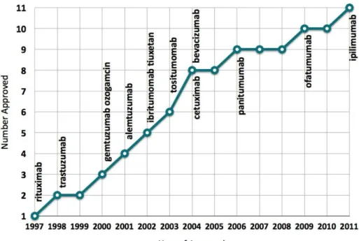
There are two main types of targeted molecular therapies. Monoclonal antibodies (O’Mahony and Bishop 2006) are usually large molecules and target (p1) and (p2) pathways (extracellular components inhibition). (For a receptor inhibition therapy study see for example Nishimoto et al. 2009). Monoclonal antibodies have protein structure, which is denatured in the gastrointestinal tract; therefore these drugs are administered intravenously. They do not have significant drug interactions, because they do not undergo hepatic metabolism. FDA (U.S. Food and Drug Administration) have approved 11 monoclonal antibodies for cancer therapy until 2011 (see Figure 2.1). The other main type of targeted molecular therapy is small molecule inhibitors. These inhibitors are smaller than antibodies, thus because of their size, they can enter cells and target (p3) and (p4) pathways (Frank2012), typically tyrosine kinase signaling (intracellular components inhibition). Small molecule inhibitors are usually administered orally rather than intravenously. Contrast to monoclonal antibodies, they undergo hepatic metabolism, so there may be drug interactions.

Targeted molecular therapies have several different types, based on specific properties of tumor development and growth.

• There are special cancer types, where tumor cells need hormones to grow. These cancers can be treated by hormone therapy. There are several ways to switch off the hormonal effects (Dinda2012): (1) prevent the body from producing and secreting the hormone, (2) block or eliminate the hormone receptors, (3) block hormone signaling pathway. The most important hormone therapies are anti- androgen therapy (e.g. against prostate cancers (Ohlmann, Kamradt, and M.

2012)), anti-estrogen therapy (e.g. against breast cancer (Verma et al. 2011)), aromatase inhibitor therapy (e.g. against breast cancer for menopausal women (Tao et al.2011)).

• Using one’s own immune system to fight cancer is calledimmunotherapy(Waldmann

(21)

Figure 2.1: FDA approved monoclonal antibodies (mAbs) for cancer therapy (Becker 2011)

2003). If the immune system has already recognized cancer cells, the immune system can be stimulated to fight more effectively against cancer (active immunotherapy).

Other solution is not to wait for immune system to recognize cancer cells, but give adequate immune system components for the patient (passive immunotherapy).

• There are already effective biological processes, where it is possible to interfere in the level of genes. Gene therapy (Kaur, Long, and Dufour2012) can be used in somatic genes (results phenotypic changes) or germ line genes (results genotypic changes).

• Revertant therapyis a potential ”natural gene therapy”, based on a newly discovered process called revertant mosaicism (spontaneous reversal of an affected somatic cell to a wild-type phenotype) (Lai-Cheong, McGrath, and Uitto2011).

• Another therapy ischeckpoint-dependent inhibition of DNA replication(Kastan and Bartek 2004), which means a cell-cycle-dependent regulation of DNA replication in tumors (Tachibana, Gonzalez, and Coleman2005).

• Apoptosis (process of programmed cell death) have key effect on tumor growth

(22)

Kasibhatla and Tseng2003).

• Antiangiogenic therapy acts against new blood vessel formation of tumor cells (see Section2.3).

The main differences between conventional cancer therapies and targeted molecular therapies are not only the acting ways, but also the goals. Using conventional treatments, there is no need to know how cancer cells are developing and which mechanisms are used to circumvent the immune system. In surgical oncology the cancer is simply removed;

radiation therapy and chemotherapy affect against rapidly dividing cells, thus these treatments are toxic to all cells. Conventional cancer therapies’ goal is to eliminate the tumor mass, but with time the tumor can recrudesce and give metastasis. Targeted molecular therapies represent a new approach: these treatments act in specific molecular ways, and the goal is to prevent tumor cells from grow and develop; hence, prevent toxicity. This is more important than eliminate the tumor mass – for the patients there is a better chance of survival if they have inactive tumor mass, than if they do not have tumor for a while, but there is the risk of recurrence. To develop targeted therapies, it is required to analyze tumor growth and explore causal factors, but with this knowledge these therapies have led to truly tailored therapy (Gerber 2008) with reduced side effects (Kreipe and Wasielewski2007).

2.3 Antiangiogenic Therapy

2.3.1 Angiogenesis

Angiogenesis is the process of forming new blood vessels, which occurs normally in the human body at specific times. During embryogenesis, blood vessels form from angioblasts (this process is called vasculogenesis). Angiogenesis also takes place in adults, although it is a relatively infrequent event (in normal circumstances occurs only in case of high altitude (low oxygen concentration), regeneration of tissue during wound healing and in women during certain phases of the menstrual cycle) (Hoeben et al. 2004). The process of angiogenesis is precisely controlled by proangiogenic and antiangiogenic factors thus as a result there is angiogenic balance in the body.

All cells need oxygen and nutrients, which can be picked up from nearby capillaries.

Tumor cells are dividing rapidly, so there is an extra need for oxygen. When proliferation begins, small sized tumor can pick up enough oxygen – in this phase tumor is an avascular nodule (dormant), in a steady-state level of proliferating and apoptosing cells (Bergers and Benjamin 2003). After a certain size (1−2 mm diameter) tumor development stops,

(23)

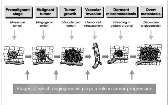
Figure 2.2: Angiogenesis in cancer development, growth, and metastasis (Hoeben et al.

2004)

because the diffusion of oxygen through tissues is limited to 100 to 200 µm. Tumor needs own blood vessels to grow, however forming new vessels is inhibited by the body’s antiangiogenic factors. Tumor have to break through this strict control – the process when tumor become able to form own blood vessels is called angiogenic switch. This switch ensures exponential tumor growth. The next phase is intravasation: the invasion of tumor cells into the blood stream. By this process, cancer cells can be spread to distant organs to form dormant micrometastases, which can induce secondary angiogenesis (Hoeben et al.

2004). Figure2.2 presents a summary of angiogenesis in cancer development, growth and metastasis.

2.3.2 Antiangiogenic Therapy

Tumor-induced neoangiogenesis is the process of forming new blood vessels by sprouting from existing vessels. After the process of forming, new blood vessels undergo changes in phenotype (this process is called vascular remodeling). These processes and thus newly

(24)

sprouting, proliferation and regression, and become dependent on VEGF (McDonald 2008). Vascular endothelial growth factor is one of the most important proangiogenic factors in tumor growth. Because of that inhibiting VEGF signaling in tumors stops sprouting angiogenesis. However, it is important to note that VEGF inhibition leads to apoptosis only in newly built vessels in tumors, but don’t have effect on vessels which have been already existing (Petersen2007).

Blood-vessel formation will continue as long as the tumor grows, therefore tumors produce VEGF constitutively. (This is why there is an expression that ”tumors are wounds that do not heal” (Hoeben et al. 2004)). VEGF circulates in the serum, thus the level of circulating VEGF is a useful marker of tumor status and prognosis in most types of human cancer (Karayiannakis et al.2002). High serum level of VEGF indicates unfavorable clinical parameters like disease progression, lack of response to chemotherapy, and poor survival (Hoeben et al.2004). A difficulty in developing antiangiogenic therapy is the monitoring of response to therapy, because decrease of tumor size is a slow process.

Nevertheless changes in hemodynamic parameters occur soon after the start of the therapy. There are several ways in medical imaging to detect these parameters’ changes (e.g. perfusion CT, perfusion MRI, contrast-enhanced ultrasound) (Kalva, Namasivayam,

and Sahani2008).

There are several angiogenesis inhibitors used in clinical application (Dredge, Dalgleish, and J. B. Marriott 2003). Research of new antiangiogenic drugs are based on the collaboration of scientists and clinicians (Kerbel and Folkman 2002). Widely used inhibitors in cancer therapies are endostatin (O’Reilly et al.1997) and bevacizumab (Ellis and Haller2008).

As it was discussed previously, targeted molecular therapies’ and thus antiangiogenic therapy’s aim is to prevent tumor cells from grow and develop, not to eliminate the whole tumor mass. If the tumor can be kept in a dormant state and the cellular proliferation rate is balanced by the apoptotic rate, the tumor will be unable to grow in size beyond a few millimeters (Pluda1997). In contrast to chemotherapy, it will not result in toxicity in the body. This characteristic is very important in cancer therapies, because a large number of cancer patients die of therapy-related toxicities, and chemotherapy can impair intellect too (this cognitive impairment is called chemobrain) (Srinivas2010). Resistance to chemotherapy is based on the genetic instability, heterogeneity and high mutational rate of tumor cells. Since endothelial cells are genetically stable, homogeneous and have a low mutational rate, antiangiogenic therapy (effecting directly to endothelial cells) induce little or no drug resistance (Kerbel1997; Boehm et al. 1997) and antiangiogenic drugs pose no risk of a chemobrain. Moreover, researches prove that antiangiogenic agents can

(25)

improve survival by increasing tolerance to chemotherapy-induced toxicity (Zhang et al.

2011).

(26)

3 Tumor Growth Model under Angiogenic Inhibition – Hahnfeldt Model

The current chapter discusses the tumor growth model under angiogenic inhibition. In Section 3.1, the nonlinear model is presented – first the original model published by Hahnfeldt et al.1999(Subsection3.1.1), and later the simplified model with which I have worked (Subsection 3.1.2). Positivity (Sub-subsection 3.1.3), equilibrium points (Sub- subsection3.1.4) and controllability of the model (Sub-subsection3.1.5) are investigated.

In Section3.2, the linearized model is presented which was created using operating point linearization (Subsection 3.2.1). Non-zero steady states and stability (Section 3.2.2), and finally observability and controllability of the linearized model (Section3.2.3) are examined.

3.1 Nonlinear Model

3.1.1 The Original Model

Hahnfeldt et al. elaborated a dynamic model for tumor growth under antiangiogenic therapy (Hahnfeldt et al.1999). In their experiments mice were injected with Lewis lung carcinoma cells. After about 3−10 days, mice were randomized into four groups. Three groups received different angiogenic inhibitors (angiostatin, endostatin and TNP-470), the fourth group was the control group (received injections of the vehicle alone).

The nonlinear model is defined by the equations:

V⁰ = −λ₁V log V K

!

(3.1) K⁰ = −λ₂K+bV −dKV^2/3−eKg(t) (3.2) g(t) =

Z t 0

c(t⁰)exp(−clr(t−t⁰))dt⁰). (3.3) The tumor growth dynamics is described by (3.1) that is a Gompertzian growth, in order to describe precisely the physiological knowledge of tumor growth slowdown.

(27)

Consequently, the state variableV is the tumor volume in mm³. The vascular support dynamics is described by (3.2), and incorporates the stimulatory effect of the tumor on vasculature support growth (with rate b), the inhibitory effect of the tumor and the vasculature (with rated), and the effect of the angiogenic inhibitor (with ratee). The state variable K is the supporting vasculature volume in mm³, and the input variable g is the concentration of the administered inhibitor in mg/kg. The third equation (3.3) incorporates the clearance of the inhibitor through a first-order system, and considers the administered inhibitor as input. Exact values of the parameters can be found in Table 3.1.

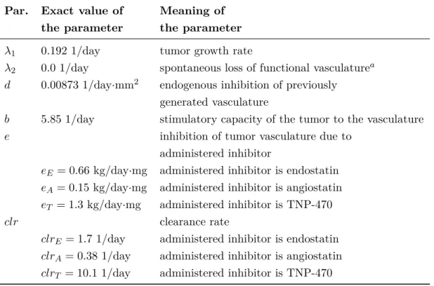
Table 3.1: Parameters of the original model of Hahnfeldt et al. 1999 Par. Exact value of Meaning of

the parameter the parameter

λ₁ 0.192 1/day tumor growth rate

λ2 0.0 1/day spontaneous loss of functional vasculature^a d 0.00873 1/day·mm² endogenous inhibition of previously

generated vasculature

b 5.85 1/day stimulatory capacity of the tumor to the vasculature

e inhibition of tumor vasculature due to

administered inhibitor

e_E = 0.66 kg/day·mg administered inhibitor is endostatin e_A= 0.15 kg/day·mg administered inhibitor is angiostatin eT = 1.3 kg/day·mg administered inhibitor is TNP-470

clr clearance rate

clrE = 1.7 1/day administered inhibitor is endostatin clr_A= 0.38 1/day administered inhibitor is angiostatin clr_T = 10.1 1/day administered inhibitor is TNP-470

a Experiments show that this parameter is always zero.

3.1.2 The Simplified Model

The original model was analyzed and transformed in several studies (d’Onofrio and Cerrai 2009; d’Onofrio, A. Gandolfi, and Rocca2009). One of the most important modifications is continuous infusion therapy (Ledzewicz and Sch¨attler 2005), where the input (the

(28)

(serum level of inhibitor), therefore (3.3) is removed from the model. Note that in the works of D. A. Drexler, L. Kov´acs, et al. 2011; D. A. Drexler, J. S´api, et al.2012, the clearance of the inhibitor is also considered.

The simplified model of tumor growth can be described by a second-order nonlinear system of differential equations (A. D’Onofrio and A. Gandolfi 2004):

x˙₁(t) = −λ₁x₁(t) log x₁(t) x₂(t)

!

(3.4) x˙₂(t) = bx₁(t)−dx₁(t)^2/3x₂(t)−ex₂(t)u(t) (3.5)

y = x₁. (3.6)

In this description x1 is the tumor volume, x2 is the endothelial volume and u is the concentration of the administered inhibitor.

This tumor growth model has some limitations. The tumor can not be totally eliminated by the angiogenic therapy in reality, the smallest achievable tumor volume is the avascular state of the tumor; however this model does not grab this phenomenon. Thus, I incorporated a lower limit of 1 mm³ into the state variables when I used the model for simulation.

Hereinafter the thesis discusses the simplified model (referred as model).

3.1.3 Positivity of the Model

Considering the real physiological system, the positivity of the model is a desirable property. Positivity means, that if the system variables are positive at an initial time t₀, then they remain positive (or nonnegative) for the whole timet≥t₀. The positivity of the system may be verified by examining the rate of change of the state variables if they are (close to) 0. If the rate of change near 0 is positive or 0, then the positivity of the state variable is guaranteed. This requires that the solution of the differential equation exists and it is continuous. These conditions are true for this model with positive initial conditions; however the proof is omitted here.

Suppose, that x₁(t₀), x₂(t₀)>0 for some initial timet₀, and examine the derivatives of the state variables at some time t≥t0. The rate of change of the tumor volume if it is close to zero is:

lim

x1(t)→0x˙₁(t) = lim

x1(t)→0−λ₁x₁(t) log x₁(t) x2(t)

!

, t≥t₀ (3.7)

(29)

that is

lim

x1(t)→0x˙₁(t) = 0, t≥t₀ (3.8)

even ifx2(t)→0 at the same time. Thus x1(t)≥0 fort≥t0. The rate of change of the vasculature support near zero is

lim

x2(t)→0x˙2(t) = lim

x2(t)→0bx1(t)−dx1(t)^2/3x2(t)−ex2(t)u, t≥t0 (3.9) that equals to

lim

x2(t)→0x˙₂(t) =bx₁(t)≥0, t≥t₀. (3.10) Thus x2(t) ≥0, for t≥t0. The positivity of the system is thus verified. Note that the positivity does not depend on the sign of the input u.

3.1.4 The Equilibrium Points of the Model

The equilibrium points of the model are the x1, x2 pairs at which the rate of change of the variables are zero. Thus the set of equilibrium points can be found by finding the solutions of

0 = −λ₁x₁log x₁

x₂

(3.11) 0 = bx1−dx^2/3₁ x2−ex2u. (3.12) The trivial solution is x₁=x₂= 0 mm³, however, since it is supposed that the initial tumor volume is not zero, and the therapy can not eliminate the whole tumor, I ignore this solution here and later. The nontrivial solution of (3.11) isx1=x2. Lety=x1 =x2

be the volume satisfying (3.11). Then (3.12) reduces to

0 =by−dy^5/3−eyu. (3.13)

Since y6= 0 mm³, this equation can be further simplified into

0 =b−dy^2/3−eu. (3.14)

Suppose, that the inputu is a constant positive value, denote this by u∞. Then the

(30)

solution y∞ of (3.14) is

y∞= b−eu∞

d

!3/2

, (3.15)

which expresses that given a constant serum level u∞, the resulting equilibrium tumor volue isy∞. Given the desired y∞tumor volume, one can calculate the required constant inhibitor serum level as

u∞= b−dy∞^2/3

e . (3.16)

This equlibrum point is asymptotically stable, since b−eu∞ is constant, and y^2/3 is strictly monotonously increasing for positivey, so the right-hand side of (3.14) is negative ify > y∞, and positive ify < y∞.

If there are no inhibitors present (u= 0), tumor and endothelial cells grow with no control input, and the steady state volume is a very high value. In this case steady state volume depends only on the type of the tumor and the patient:

y∞= b d

!3/2

. (3.17)

Tumor growth without antiangiogenic therapy leads to high steady state tumor volume (y∞ = 1.734·10⁴ mm³) and it represents the lethal steady state case (upper part of Figure3.1). Using angiogenic inhibition, tumor size can be reduced from a high tumor volume to a low value. In the lower part of Figure 3.1 the effect of constant 5 mg/kg endostatin inhibition was simulated.

3.1.5 The Controllability of the Model

In the previous subsection the static behaviour of the system was analyzed. Using (3.16), one can calculate for example the amount of inhibitor needed to maintain the tumor in avascular state. However, equations (3.15) and (3.16) does not take the dynamics of the system into consideration. By applying the results of control engineering, we can affect the dynamics of the system that is the speed and characteristics of the tumor volume decreasing to the avascular state.

In order to apply control techniques, the controllability of the model needs to be checked. In this subsection the analyzis of controllability using the Lie Algebra Rank Condition (LARC) is performed (Isidori1995).

The tumor model is a nonlinear, input affine, single input single output (SISO) system

(31)

0 20 40 60 80 100 0

0.5 1 1.5

2x 10⁴

Time [day]

Volume [mm3]

Tumor growth without antiangiogenic therapy

tumor volume without therapy vascular volume without therapy

0 20 40 60 80 100

0.5 1 1.5

2x 10⁴

Time [day]

Volume [mm3]

Tumor regression using constant (5 mg/kg) inhibitor dosage

tumor volume using constant therapy vascular volume using constant therapy

Figure 3.1: Tumor growth without angiogenic therapy (upper figure) and under constant angiogenic inhibition (lower figure)

that can be written in a general form as

x(t)˙ = f x(t)+g x(t)u(t) (3.18)

y(t) = h x(t). (3.19)

In the current application, the drift vector field atx is

f(x) =







−λ₁x1log x1

x₂

bx₁−dx^2/3₁ x₂







, (3.20)

(32)

the control vector field at the point xis

g(x) =





 0

−ex₂





, (3.21)

and the output vector field atx is

h(x) =x₁. (3.22)

The nonlinear system is controllable, if the Lie algebra generated by the control and drift vector fields span the whole state space. Thus it is needed to check whether g and the Lie bracket of f andg are linearly independent. The Lie bracket of two vector fields at the point x is

[f, g] (x) = (∂_xf)(x)g(x)−(∂_xg)(x)f(x). (3.23) The Lie bracket of the vector fields f and g at the point at is thus

[f, g] (x) =







−λ₁ex1

bex₁





. (3.24)

The linear independence of g and [f, g] can be checked by examining the rank of the matrix valued function ∆ with columns g and [f, g]:

∆(x) =







0 −λ₁ex₁

−ex₂ bex1





, (3.25)

that has the determinant

det ∆(x)=−λ₁e²x1x2. (3.26) The matrix ∆(x) is full rank, whenever its determinant is not zero. From (3.26) the determinant is zero if a) x1 = 0 mm³, however this case was already excluded; or b) x₂ = 0 mm³. In these situations the model is not controllable. Note that ifx₂ = 0 mm³, then the tumor is in the avascular state, and the input required to maintain the tumor in that state can be calculated using the static equation (3.16). Note that ∆(x) has the same image space as the linear subspace spanned by controllability Lie algebra (Isidori 1995), thus the system is controllable in every point xwhere (3.26) is not zero. We can now conclude that the nonlinear model of tumor growth is controllable wheneverx1 6= 0 mm³ and x₂ 6= 0 mm³.

(33)

3.2 Linear Model

3.2.1 Operating Point Linearization

The tumor model is nonlinear, but the control techniques I apply later are linear, thus a linear approximation of the tumor growth model is needed for design purposes. A linear dynamic model is usually written in the form

x(t)˙ = Ax(t) +Bu(t) (3.27)

y(t) = Cx(t) +Du(t), (3.28)

where (3.27) defines the dynamics of the system, and (3.28) defines the output of the system. The linear approximation of the tumor growth model is acquired by first-order approximation at specific operating pointx and u= 0 mg/kg, i.e.

A(x, u) = ∂x(f +gu)(x, u), (3.29) B(x, u) = ∂u(f +gu)(x, u), (3.30)

C(x, u) = ∂x(h)(x, u), (3.31)

D(x, u) = ∂_u(h)(x, u), (3.32)

which yields in this special case

A(x) = (∂_xf) (x), (3.33)

B(x) = g(x), (3.34)

C(x) = (∂xh) (x), (3.35)

D(x) = 0. (3.36)

(34)

The matrices of the linear model acquired at the operation point xare

A=







−λ₁·log^x_x¹

2

−λ1 λ1x1

x2

b−²₃d·x⁻

1 3

1 ·x2 −d·x

2 3

1







(3.37)

B =





 0

−ex₂







(3.38)

C =

"

1 0

#

(3.39) D=

"

0

#

(3.40) The vector x is chosen such that both of its components are equal. Let x12 be the value of the tumor volume at the operating pointx, then the vector x isx= [x₁₂, x₁₂]^>. 3.2.2 Non-Zero Steady States and Stability of the Linearized Model

As it was discussed in Subsection3.1.4, if the system is in steady state (the system is in an equilibrium point), tumor volume and vascular volume are equal (x₁=x₂). Let this steady state volume bex₁ =x₂=x₁₀. Then the system matrix A(3.37) reduces to

A∞=







−λ₁ λ1

b−²₃d·x

2 3

10 −d·x

2 3

10



