BH N
O CC ASIONAL P A PE R
8 S
The monetary programme
(A methodological description)
and do not necessarily represent those of the National Bank of Hungary
Compiled by: Gyula Barabás–Klára Major
members of the Monetary Policy Department of the National Bank of Hungary Tel.: 36–1–302–3000/2344, 2050
E-mail: barabasgy@mnb.hu. majork@mnb.hu
Issued: by the Department for General Services and Procurement of the National Bank of Hungary Responsible for publishing: Botond Bercsényi
8–9 Szabadság tér, H-1850 Budapest Prepared for publication by the Publications Group
Mailing: Miklós Molnár Internet: http://www.mnb.hu
ISSN 1216-9293 ISBN 9637103899
1. Major concepts of the monetary programme · · · 5
1.1 Net financing capacity · · · 5
1.2 Nominal and operational flows · · · 7
2. Calculating financing capacity · · · · 10
2.1 The current account and components of its financing · · · 10
2.2 Net financing capacity of general government · · · 11
2.3 Net financing capacity of the household sector · · · 13
2.4 Net financing capacity of the corporate sector · · · 13
2.5 The flow-of-funds matrix · · · 17
3. Stages of constructing the monetary programme · · · · 18
3.1 Forecasting financing capacity · · · 18
3.2 Consistency of data of the financing and income sides · · · 21
3.3 Foreign exchange market intervention and its components· · · 23
3.4 Flow of funds: consistency at the level of instruments · · · 32
4. Forecasting monetary aggregates · · · · 33
4.1 Aggregate balance sheet of the banking sector · · · 33
4.2 Balance sheet of the central bank · · · 34
4.3 Rolling liquidity programme · · · 35
Appendix 1:Flow-of-funds matrix· · · 39
Appendix 2:Flow-of-funds matrix on the basis of 1999 values · · · 40
Appendix 3:Stages of constructing the monetary programme · · · 41
Appendix 4:Rolling liquidity programme · · · 42
Appendix 5:Variables· · · 43
Contents
The forecast horizon is 8–17 months
A
monetary programme is constructed every three months by the Monetary Policy Department staff of the National Bank of Hun- gary. Based on the Economics Department’s projections of several key macroeconomic variables, the programme is constructed after several rounds of discussion between the two departments. The time horizon of the projections varies between 8 months and 17 months.By way of example, when constructing the April monetary programme, the focus of the forecast is usually on the current year.
The July monetary programme, however, takes a broader perspec- tive, as it includes projections for the following year as well.
1.1 Net financing capacity
Net financing capac- ity = income – con- sumption – accumulation
The Monetary Programme provides a method of forecasting the net financing capacities of the individual institutional sectors, the key monetary aggregates, the balance sheet of the central bank and the consolidated balance sheet of the banking sector. A sector’s net fi- nancial savings, i.e. the portion of its income that it does not spend on consumption or accumulation, is generally referred to asnet fi- nancing capacity.2Net financial savings of one sector thus provide a source of spending by some other economic unit over and above its income.Therefore, the sum of net financing capacities of all resi- dent and non-resident units is equal to zero– if one sector utilises its resources on consumption and accumulation in excess of its in- come, it can either finance the resulting gap by disposing of its as- sets or by borrowing from other sectors. This then will cause its net financing capacity to become negative, which will be counterbal- anced by the positive overall net financing capacity of other sectors.
1The authors would like to thankIstván Ábel, Emma Boros, Tamás CzetiandPéter Koroknaifor their assistance in writing this Paper. Our thanks also go to the participants in the discussion of the first draft held at the Bank for their valuable comments. Naturally, it is the authors who should be held responsible for any occurrence of error. This analysis reflects the authors’ views, which do not necessarily correspond to the official viewpoint of the Bank.2
If an economic agent spends more than its income, its net financing capacity is negative. This is referred to as a borrowing requirement. Positive net lending capacity is also referred to as financing capacity.
1| Major concepts of the monetary
| programme1
The monetary programme provides a description of the major financial and income trends of the four institutional sectors, i.e. the corporate, household, general government and non-resident sec- tors. Net financing capacities are calculated for these four sectors.
However, because they develop rather differently, the positions of the financial and non-financial corporations sub-sectors within the corporate sector are shown individually(see Table A).
Net financing capac- ity can be derived from both the financ- ing and income sides
Net financing capacity can be derived from boththe financing and income sides. In the first case, net financing capacity can be measured by analysing changes in financial assets and liabilities, i.e.
financial wealth of the individual sectors. In the second case, the in- dicator is calculated by describing the path of the individual sectors’
incomes, the application of their incomes and subtracting consump- tion and accumulation expenditures of sectors from their respective incomes. Despite the differences in these approaches, the methods of deriving net financing capacity should produce the same result, providing a framework for cross-checking the forecasts.
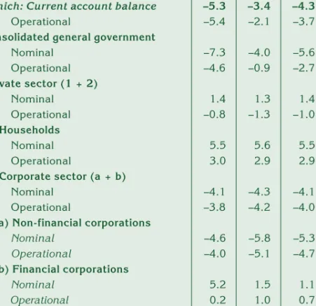
Table A Net financing capacity of the individual sectors; as a percentage of GDP
1999 2000
H1 H2 H1+H2 H1
Net foreign borrowing requirement (I + II)
Nominal –5.9 –2.7 –4.3 –3.3
Of which: Current account balance –5.3 –3.4 –4.3 –3.6
Operational –5.4 –2.1 –3.7 –2.6
I. Consolidated general government
Nominal –7.3 –4.0 –5.6 –4.4
Operational –4.6 –0.9 –2.7 –1.1
II. Private sector (1 + 2)
Nominal 1.4 1.3 1.4 1.1
Operational –0.8 –1.3 –1.0 –1.5
1. Households
Nominal 5.5 5.6 5.5 4.5
Operational 3.0 2.9 2.9 2.0
2. Corporate sector (a + b)
Nominal –4.1 –4.3 –4.1 –3.4
Operational –3.8 –4.2 –4.0 –3.4
a) Non-financial corporations
Nominal –4.6 –5.8 –5.3 –5.3
Operational –4.0 –5.1 –4.7 –4.4
b) Financial corporations
Nominal 5.2 1.5 1.1 1.8
Operational 0.2 1.0 0.7 1.0
1.2 Nominal and operational flows
Change in stock – other volume change – exchange rate effect
= nominal flow
Forecasts of changes in financial assets and liabilities take flows, that is ‘net’ changes in stocks due to transactions, as their point of origin. The reason for choosing this approach is that changes in stocks also include the effects of factors which tend to increase the difficulty and uncertainty in exploring the underlying developments which need to be grasped in order to produce the projection. There- fore, in constructing the monetary programme, so-callednominal flows3are determined from the changes in stock data by eliminating the effects of both exchange rate movements and other changes in the volume of assets and liabilities (only the effect of other volume changes in respect of forint-denominated financial assets).4
Nominal flow – com- pensation for inflation
= operational flow
A nominal flow for a given stock of assets includes (nominal) interest payments on financial assets as well as changes due to transactions other than interest payments.5The real return on a fi- nancial asset is derived by eliminating the impact of inflation on the nominal return. The sum of real return and changes in the volume of financial assets due to transactions other than interest payments is calledoperational flow (see Table B), which, unlike the nominal flow, does not reflect the distorting impact of inflation. In this manner we obtain an indicator which can help us to explore the underlying de- velopments in the individual sectors’ net financing capacities, even in an environment characterised by high and variable inflation.
Operational flow does not include the dis- torting effects of infla- tion
In calculating operational flow, the lower of nominal interest and the inflation rate,6is used to derive compensation for inflation.
This means that, when calculating operational flows, the real interest component, added to the value of transactions other than interest payments, is positive if the interest rate on the asset is higher than the rate of inflation and, conversely, is zero if the interest rate is lower than inflation.
3Our use of the various concepts differs from that of the SNA, where flows include the effect of exchange rate changes, in addition to that of transactions.4
Other volume effect, e.g. the write-off of a loan, when the amount of outstanding debt changes without a transaction taking place.5
Transactions other than interest payments mean net purchases and deposits in the case of assets, and net borrowing in the case of loans.6
When calculating operational flows, compensation for inflation is subtracted from interest or in- terest type income earned on financial assets. This means that, in addition to bank deposits and lending, compensation for inflation is also computed in the case of investment funds investing in government debt securities. However, the value of compensation for inflation is zero the case of non-interest-bearing cash investments and acquisitions of shares not guaranteeing secure returns.
Table B Relationship between nominal and operational flows
Nominal flow
Interest income Transactions other than interest payments Compensation for inflation Real interest
rate Transactions other than interest payments Compensation for inflation Operational flow
When inflation exceeds the nominal return on an asset, the in- vestor earns negative real interest by holding various financial as- sets. Negative transfers of income between issuers of a financial as- set and holders, which arises in economic terms, is not taken into ac- count in determining operational flows. The reason for this is that the international statistical system (SNA) also uses this indicator, thus enabling us to obtain internationally comparable data.
Another argument for calculating the operational flow with the above approach is that taking account of negative interest income would cause complications when recording the income of the indi- vidual sectors. The operational net financing capacities of the vari- ous sectors include an amount of disposable income which, when the sector’s consumption and accumulation expenditure is sub- tracted, provides us with the sector’s net financing capacity. If nega- tive real interest were taken into account when calculating opera- tional flows and financing capacity, a transfer of income which is both difficult to statistically interpret and which does not involve gen- uine financial flows would have to be recorded on the income side.
Different categories of income are associ- ated with nominal and operational flows
There is also a disposable income component of operational fi- nancing capacity which is associated with zero or positive real inter- est. This is obtained by subtracting the compensation-for-inflation component of interest and interest type incomes from the disposable income component of nominal net financing capacity. This allows the process of adjusting for inflation to be interpreted in the in- come-side approach as well, and thus operational financing capac- ity can be calculated from both the perspective of income and fi- nancing.
Nominal income, which is consistent with nominal flows, can primarily be disaggregated into labour and property income constit- uents. The latter constituent also includes interest type income. This implies that interest income, calculated on the basis of the nominal interest rate, not only includes the real income of a given sector, but compensation for the diminution in the value of a financial asset caused by inflation as well. In estimating the incomes pertaining to the operational borrowing requirement of specific sectors, this com-
Table C Relationship between nominal and operational income
Nominal income
Property income Labour income
Interest income Allowances Labour income
Compensation for inflation Real interest rate Allowances Labour income Compensation for inflation Operational income
pensation component must be eliminated. Consequently, in the op- erational approach, income is derived by subtracting the inflation compensation component of nominal interest from property income (see Table C).
The first step is to pro- duce the forecast of operational financing capacities
When constructing the monetary programme, the first step is to produce forecasts of the individual sectors’ operational financing ca- pacities and to project the operational flows of the various assets and liabilities. These indicators are then modified by the inflation- compensation component on the basis of forecast inflation. This provides us with forecasts of both nominal financing capacities and changes in stocks. However, both calculations, i.e. the programme based on nominal flows and that based on operational flows, must concur with developments on the income side. At the same time, by ensuring this consistency both approaches can be cross-checked.
Forecasting financing capacities is not ag- gregating financial
assets
T
his Section describes the method of estimating the individual sectors’ net financing capacities by deriving from the financing side. The equations referred to present a detailed explanation of how net financing capacity can be calculated for each sector, based on fi- nancial assets and liabilities and on the various items in the balance of payments. Later on, we will present in detail the steps of construct- ing the monetary programme itself. We should like to emphasise, however, at this early stage that, in generating the prognosis, the monetary programme is not constructed as an aggregation of the in- dividual forecasts of various financial assets. On the contrary – the decisions taken by the individual sectors in respect of their portfolios, that is, the expected measure of changes in the individual items of wealth, is determined using net financing capacity as a basis.2.1 The current account and components of its financing
The monetary programme states the individual sectors’ net financ- ing capacities on a cash basis instead of an accrual basis. The net external borrowing requirement is therefore equal to the sum of the current and capital account deficits.
The following items constitute the major components of the balance of payments:7
– Current account balance (CA);
– Capital account balance (KA);
– Foreign direct investment (excluding privatisation revenue, FDI);
– Foreign borrowing: credit flows of consolidated general gov- ernment, i.e. the NBH and the central government (DLFG= DLFJ+DLFK),8foreign borrowing by the non-financial corpora- tions sector (DLFV) and foreign borrowing by credit institu- tions (DLFB);
2 | Calculating net financing capacity
7The variables used in the description are included in the Appendix at the end of the document.
8Here and in the following,Dis meant to indicate the change in the volume of a given instrument after eliminating the effects of exchange rate movements and other volume changes, i.e. nominal flows. The relationships are valid using operational numbers as well. In this case, changes in stocks
– Acquisitions of government securities (DBF) and shares (DEF, including foreign currency revenue from privatisation) by non-residents; and
– Changes in international reserves (Res).
Using these items, the current account equation can be ex- pressed as follows:
CA+KA+FDI+DLFG+DLFV+DLFB+DBF+PvF+DEF=DRes (1) Rearranging equation (1), we obtain the items financing the current account deficit(see Table D).9
2.2 Net financing capacity of general government
General government consolidated with NBH
In order to estimate the general government net borrowing require- ment, the change in the debt ofconsolidated general government, including the central bank, is determined as a first step. In this con-
9In each case, the quantification of the various equations has made it necessary to include an item, so as to be able to handle data errors and other discrepancies. This error component, how- ever, is not shown separately in the equations.
Table D Current account formula (1998, 1999 and 2000 H1)
millions Variables 1998 1999 2000
H1 1. Current account balance CA –2,020 –1,970 –860
2. Financing 2,780 4,212 983
2.1Foreign direct investment
(net of privatisation revenue) FDI 1,387 1,612 906 2.2Credit balance of consolidated
general government DLFG 276 1,219 –2
Credit balance of NBH DLFJ –400 –1,657 –807 Credit balance of central government
(excluding government securities) DLFK –119 2,274 223 Acquisitions of government securities
by non-residents DBF 795 601 583
2.3Privatisation revenue PvF 158 351 8
2.4Net borrowing of the private sector 761 1,236 41 Borrowing of credit institutions DLFB 311 299 715 Portfolio investments
(net of privatisation revenue) DEF 302 608 –289 Corporate foreign borrowing DLFV 148 329 –385
2.5Capital account balance KA 170 31 84
2.6Balance of errors and omissions 28 –237 –54 3. Change in international reserves DRes 760 2,241 123
solidation, the mutual assets and liabilities of general government and the central bank are eliminated, but at the same time assets and liabilities of the central bank vis-à-vis non-residents and the domes- tic private sector are included. The required reserves of commercial banks appear as a constituent of the monetary base, and their two-week deposits with the NBH are treated as part of sterilisation instruments, similar to the treatment of NBH bills(see Table E).
Privatisation reve- nues treated as a cor- rection item
When we express the sector’s net borrowing requirement based on the consolidated general government balance sheet presented in Table E, state property must also be shown on the asset side of the consolidated general government balance sheet. The reason for tak- ing this approach is that proceeds from privatisation result in a de- crease in state ownership, which is presented on the assets side of the general government balance sheet. When state assets are sold, government ownership declines (Pv = –DEG), but general govern- ment’s net financial assets increase, and the transaction leaves the sector’s net financing capacity unaffected. Net financing capacity, calculated on the basis of net financial assets, but taking no account of revenues from privatisation, would show the position more favour- ably than it actually is. Therefore, when calculating net financing ca- pacity, privatisation revenues are taken into account with a negative value, as an item increasing the borrowing requirement.
NFKG= –DKP –DRR –DB –DLFG–DCDFt–DCD$– Pv +DRes +DLJB(2) In order to forecast the central bank balance sheet, one of the pillars of the monetary programme, it is necessary to produce the asset and liability statements of the central bank and general gov- ernment (the two sub-sectors of the consolidated general govern- ment sector) separately. Therefore, given that the simplified flow- of-funds matrix in Appendix 1 to this Paper includes the various items in a breakdown by sub-sector, the mutual assets and liabilities
Table E (Simplified) balance sheet of consolidated general government
Asset Liability
LJB Refinancing loans Monetary base (banknotes and coin
plus required reserves) KP+RR Res International reserves Outstanding sterilisation instruments CDFt
EG Equity ownership Foreign currency deposits of commercial banks
CD$ Foreign borrowings of general
government LFG
Outstanding government paper B
of the two sub-sectors are also indicated. Among these items, the most important ones are the government’s account held with the central bank (the Treasury Account) and net foreign currency lend- ing by the central bank to the government (DLJK$ ). (The latter in- cludes the government’s special foreign currency deposits with the central bank, with a negative sign.)
2.3 Net financing capacity of the household sector
The calculation of household sector net financing capacity takes into account the following financial assets:
– cash holdings (DKPH);
– forint deposits (DDHFt); these include outstanding bank secu- rities and the sector’s assets in home-savings institutions as well;
– foreign currency deposits (DDH$);
– government securities holdings (DBH); and
– holdings of securities issued by enterprises, whereby claims on company equity (shares, DEH)10 are distinguished from claims on financial corporations other than credit institutions (investment fund certificates, life insurance reserves, the sec- tor’s equity in pension funds,DMF).
The vast majority of household sector financial liabilities are accounted for by commercial bank lending (LBH). Taking into view all these, net financing capacity, i.e. the increase in net financial as- sets, can be expressed by the following formula:
NFKH=DKPH+DDHFt +DDH$ +DBH+DEH+DMF –DLBH (3)
2.4 Net financing capacity of the corporate sector
Financial and non-financial corpo- rations should be treated separately
When analysing the corporate sector, companies are categorised into those pursuing financial and non-financial activities. In addi- tion, credit institutions are also treated separately within financial corporations, by virtue of the role they play in the economy.
10Currently, this primarily indicates holdings of exchange-traded shares. However, as there is no available statistical information regarding shares outside the Stock Exchange, we are unable to give an accurate forecast of the sector’s holdings of shares.
2.4.1 Non-financial corporations
The definition of non-financial corporations’ net financing capacity is similar to that of the household sector. The following asset catego- ries comprise the sector’s financial assets:
– cash holdings (DKPV);
– forint deposits (DDVFt);
– foreign currency deposits (DDV$);
– government securities holdings (DBV);
– holdings of NBH bills (DCDVFt) and – equity ownership (DEV).
Corporate sector financing can be categorised into the follow- ing components:
– issues of shares (IV);
– increase in forint borrowings from domestic credit institutions (DLFtBV);
– increase in foreign currency borrowings from domestic credit institutions (DLBV$ );
– increase in foreign currency borrowings from abroad (DLFV);
– andforeign direct investment (FDI).
Based on these items, the net financing capacity of non- financial corporations can be expressed as follows:
NFKV=DKPV+DDVFt DD
+ V$ +DBV+DCDVFt +DEV– – IV–DLFtBV –DL$BV – DLFV– FDI (4)
2.4.2 Financial corporations
Credit institutions within the financial corporations sector are given a special role
The expression defined by formula (4), does not represent the entire corporate sector’s financing capacity: the net financing capacity of financial corporations must also be added. Financial corporations can be disaggregated into two further sub-groups, namely (1) credit institutions and (2) financial corporations. This grouping is justified by the fact that key items in the balance sheets of credit institutions are afforded a special role in the monetary programme when fore- casting the aggregate balance sheet of the banking sector.
In respect of the corporate sector, accumulation expenditure, i.e. fixed investment and increase in inventories, typically occurs outside of the financial sector. Therefore, in analysing the financial sector, a simplifying assumption has been made that the sector does not spend on accumulation, so its net financing capacity is de-
pendent on profits earned. Profits of the financial sector can be closely linked to its disposable income, which, if positive, increases the total available income of domestic sectors and reduces the coun- try’s external borrowing requirement. Basically, the financial sector links parties with financial savings to borrowers. Nevertheless, the sector is capable of lending in excess of the value of the financial savings it attracts, up to the extent of its disposable income.
In accordance with the method of calculation from the financ- ing side, the change in net assets, after elimination of the effects of exchange rate movements and other volume effects, must show the net financing capacity (or, for the sake of simplicity, profits) of the fi- nancial sector, as is the case in respect of other sectors. Therefore, in order to derive net financing capacity we must take the balance sheet of the financial corporation sector as a basis, and calculate such capacity from changes in the sector’s financial assets and lia- bilities.
2.4.2.1 Credit institutions
The net financing capacity of credit institutions is defined with due consideration of the following classes of financial assets and liabili- ties(see Table F).
Table F Aggregate balance sheet of credit institutions
Asset Liability
KPB Cash Shareholders’
quality
CB
RR Required reserves Forint deposits DFt= DVFt+DHFt+DRFt CDFt Forint deposits with
central bank Foreign currency
deposits D D D$= V$+ H$
CD$ Foreign currency deposits with central bank
Refinancing
loans LJB
L LBFt L L
FtBH BVFt
BRFt
= + + Forint lending Foreign borrow- ing of commer-
cial banks LFB
LBV$ Foreign currency lending
CBB Corporate bonds BB Outstanding govern-
ment paper
Accordingly, the increase in the net assets of credit institutions can be expressed with the following formula:
NKFB=DKPB+DRR +DCDFt+DCD$+DLFtB DL
+ $BV +DBB
– IB–DDFt –DD$–DLJB–DLFB (5)
where the change in shareholders’ equity equals the value of shares issued by credit institutions:DCB=IB.
2.4.2.2 Other financial corporations: investment funds, insurance companies, securities brokers
Other financial corporations are categorised into one sub-sector. In addition to investment funds, this sub-sector also includes insur- ance companies and pension funds. In determining this sub-sector’s net financing capacity, the following financial assets and liabilities are taken into account:
– government securities holdings (DBR);
– forint deposits (DDR);
– holdings of NBH bills (DCDRFt)
– forint borrowings from domestic banks (DLBR);
– acquisitions of equity stakes in non-financial corporations (total holdings of corporate shares,(DER);and
– major liabilities of the sector: outstanding investment fund certificates, life insurance reserves, liabilities of pension funds to the household sector (DMF).
Using these items, the formula for determining their net financ- ing capacity can be expressed as follows:
NKFR=DDR+DBR+DER+DCDRFt –DMF –DLBR (6) Total corporate sector net financing capacity is the sum of the three sub-sectors’ net financing capacities taken individually. Using formulae (4), (5) and (6), this can be expressed as follows:
NFKTV= NFKV+ NFKB+ NFKR (7) As well as providing a description of credit flows between the sub-sectors, the simplified flow-of-funds matrix is an important ele- ment in estimating the net financing capacities of the individual sub-sectors, and summarises the interrelationships presented so far.
2.5 The flow-of-funds matrix
Changes in assets and liabilities of the four sectors are pre- sented by the flow-of-funds matrix
The flow-of-funds matrix we employ, which is constructed from mu- tual assets and liabilities of the individual sub-sectors, is presented in Appendix 1.11Changes in the financial assets and liabilities of the four sectors constitute a closed system – every financial asset is si- multaneously a liability of another sector. Consequently, if for a given asset we aggregate the changes in stocks at the levels of the individual sectors by assigning positive value to an increase in as- sets and negative value to an increase in liabilities the result is zero.
It follows that the sum totals of the items in the individual rows of the flow of funds matrix must be zero.
As the asset and liability portfolios are mapped out separately for each sector, when constructing the monetary programme, the flows must be analysed in a closed system in order to ensure consis- tency. The flow-of-funds matrix describes market participants’ deci- sions on their asset and liability portfolios in such a way which en- sures the equilibrium of money and capital markets, that is, the bal- ance of supply and demand for financial assets.
Supply of and de- mand for the individ- ual instruments are equal
The flow-of-funds matrix, therefore, complements the relation- ship presented earlier,according to which the sum of net financing capacities of the individual sectors is zero, with further equations re- lating to the individual instruments.
Sum of net financing capacities of the sec- tors is zero
The products of the money, foreign exchange and capital mar- kets have been categorised into 11 groups, according to their inter- est-bearing nature and characteristic yield levels (financial assets shown in rows 1–11 of Appendix 1). The breakdown of product groups according to different liquidity characteristics and currency denomination is mainly justified by the fact that this presents a suffi- ciently detailed picture of market participants’ portfolio-based asset allocation, while also providing an opportunity to calculate the major financial and credit aggregates.
The next four rows (12–15) detail all those major financial asset classes which are indispensable ingredients for forecasting the cen- tral bank balance sheet, and which are not included in the monetary aggregates. They include financial settlements between the central government and the central bank and those between the central bank and commercial banks. In the system provided by the flow-of-funds matrix, equilibrium is established between the balance sheets of the central bank, the banking sector and the major institu- tional sectors at the levels of both the sectors and the instruments.
Appendix 2illustrates a version of the flow-of-funds matrix as- sembled on the basis of actual data for 1999.
11In the flow-of-funds table, changes in liabilities of a sector is shown with a negative value and those in assets with a positive value.
Step 1: forecasting fi-
nancing capacities
T
he flow chart for constructing the monetary programme and the synopsis of the individual steps to be taken are presented inAp- pendix 3.The following is a step-by-step description of the proce- dures followed, according to the matrix shown in the Appendix. The first step consists of determining the financing capacity of the vari- ous sectors. In order to do this, developmentsin the short-base trend, obtained by assembling past data for net financing capacity and analysing its series, forecasts of GDP, inflation and the interest rate path as well as of the state budget, are used as inputs. The final val- ues for net financing capacity are determined taking into account economic events on the income side and by providing for consis- tency between the financing and income sides.Step 2: forecasting fi-
nancial assets When the net financing capacities of the various sectors are known, the financial assets that underlie the changes in financial wealth of the individual sectors can be identified using portfolio anal- ysis. During this phase of constructing the flow-of-funds matrix, disaggregation of foreign exchange market intervention into its con- stituents and analysis of the interrelationships between the current account, foreign exchange market intervention and the central bank balance sheet play an important role.
Step 3: assembling the consolidated bal- ance sheet of the banking sector and the rolling liquidit
Given the changes in the various financial assets, we are now able to assemble the consolidated balance sheet of the banking sec- tor and, finally, the rolling liquidity programme is also constructed.
This Section provides a more detailed overview of the process of forecasting net financing capacity, the interrelationships between the balance of payments, foreign exchange market interventions and the central bank balance sheet as well as the construction of the flow-of-funds matrix. The balance sheets and rolling liquidity programme, representing the outputs of the monetary programme, will be presented in the next Section.
3.1 Forecasting net financing capacity
The structure of the forecast is built on the flow-of-funds matrix. The essence of this is that the net financing capacities of the three sec- tors comprising the economy, i.e. general government, enterprises
3 | Stages of constructing the monetary
| programme
and households, and of non-resident sector can be encapsulated in a closed system. The objective of the monetary programme is to formulate the structure of assets and liabilities of the sectors so that the assets and liabilities with various liquidity and currency denomi- nation characteristics each constitute a closed system as well.
Seasonally adjusted operational flows serve as basis for the forecast
Operational flows, which better reflect the underlying develop- ments and are adjusted for inflation, serve as a basis for producing the forecast. Generally, economic transactions reflect significant seasonal influences, therefore, when possible, seasonally adjusted data are used, which are transformed into data on a constant price basis for the purpose of comparing such with past events. Taking these steps we obtain the time series for the sectors’ assets and lia- bilities which can be interpreted from an economic perspective. Oc- casionally, these data, which are collected on a monthly basis, ex- hibit strong fluctuations: in such cases the values are smoothed us- ing moving averages. This allows economically justifiable develop- ments to become more evident.
A wide range of data, for example the inflation path and the first draft of the GDP forecast by the Bank’s Economic and Research De- partment, is used as exogenous factors to produce the forecast. Sim- ilarly, the financing capacity of the general government sector can also be viewed as an exogenous factor.
Time series analysis and stability test
Given the lack of formalised relationships, items on the financ- ing side are forecast using several methods. The first phase of pro- ducing the projection is time series analysis. Seasonally adjusted time series of operational flows, which eliminate the distorting effects of inflation, are calculated for both financing capacities and individ- ual assets. Within the framework of the time series analysis, the autoregressive (in most cases ARIMA) model, as employed by the Demetra programme,12produces the future trend of a given variable which can be adjusted for seasonality. Based on this trend the future values, as estimated by the Demetra programme, can be derived by adding the seasonal factors. These projections represent an impor- tant starting-point for forecasting the financing items.
The reliability of the figures projected for the various time series by Demetra varies. Therefore, in each case we analyse the stability of the trend forecast by the programme, i.e. whether it changes sig- nificantly when new data is entered. One possible method of con- ducting this stability measurement exercise is to set, for a given point in time, the autoregressive model and its parameters found optimal by Demetra, and test whether the time series complemented with new data can be reconciled with the model expressed on the basis of earlier data. If the expanded time series cannot be explained by the fixed model on the basis of the significance tests, this suggests a cer-
12The Demetra programme, designed for Eurostat, runs the TRAMO & SEATS and X-12-ARIMA algorithms for seasonal adjustment to analyse the individual time series. Our analyses have been made using Version 1.4 of the programme, released in February 2000.
tain instability. In this case, forecasts produced by Demetra should be treated with reservation.
If the time series does not show the effect of any significant sea- sonal pattern (for example, foreign capital inflow), the time series forecast by Demetra is not available. In such cases, the original times series are analysed using other methods, for example moving averages, in order to reveal both short-term and future trends. The use of moving averages may be useful in the case of seasonally ad- justable time series, if the seasonally adjusted time series is ex- tremely volatile and the trend calculated by Demetra is unstable, that is, it reacts sensitively to new data.
Finding explanatory variables using corre- lation calculations and simple regres- sions
In addition to the time series analysis, identifyingexplanatory vari- ableswhich could, in theory, affect the given flow and developments in the value of a given asset is an important step in the forecasting pro- cess. As regards the variables which may, in theory, be used for the analysis, it is analysed for which variables thecorrelation calculations and simple regressions indicate a statistically significant relationship, pointing in the same direction with that expected on the basis of theory.
Due to the structural disruptions caused by economic transi- tion, the short time series and errors in the statistical data, we have not found yet an econometric model, the parameters of which could be safely relied upon in formulating projections. So far, the most reli- able results have been achieved when explaining the behaviour of cash holdings. In respect of most items, the significant effect of one or more variables is demonstrable on the basis of the correlation cal- culations. Nevertheless, we have not yet been able to generate re- gressions which are able to satisfy serious stability tests. In these cases, either the theoretically expected coefficient is hypothesised (for example, 1 in the case of elasticity of the real quantity of money according to income) or an analysis is conducted to determine whether the projection using parameters suggested by the simple re- gressions passes the wide variety of consistency tests required by the relationships of the monetary programme.
Past data do not appear to confirm the theoretically expected relationships for certain instruments. In this case, if a given explana- tory variable is expected to show considerable variation based on the forecasts of inflation and yields on the income side, this is taken into account when projecting operational flows. As the coefficient of the explanatory variable is unknown, this means that, within the bound- aries defined by the consistency analyses, the forecast is modified to a greater or lesser extent in a certain direction which is theoretically justified by the future shifts in the explanatory variable.
Income-side variables and the inflation fore- cast are produced by the Economics and Research Department
The forecast of variables explaining the items on the financing side is founded on the projections of changes in the income side and inflation contributed by the Economics and Research Department.
The most important explanatory variables derived from such are the
individual sectors’ disposable income and the various components of GDP (consumption, fixed investment, net exports), as well as in- flation. In addition, the monetary programme renders forecasts for the future path of three-month government securities yields using in- formation derived from the yield curve, and the expected future tra- jectory of interest rates on loans and deposits as well. The transmis- sion relationship between the three-month government securities yield and interest rates on loans and deposits allows us to forecast lending and deposit rates with relative accuracy. This forecast, in turn, will play a role as an explanatory variable when forecasting op- erational flows.
The values derived from forecasting the financing capacities of the four sectors, i.e. non-residents, general government, households and enterprises, are very closely interlinked, which allows us to cross-check and modify the plausibility of net positions which reflect developments characteristic of a given sector. During this cross- checking, the figures on the financing side are checked against the first draft of the forecast obtained from the income-side analysis, which uses the same figures for growth and balance of payments, and final projections ensuring the consistency of the two sides are then formulated. A detailed description of the process of establishing the consistency of the data on the income and financing sides is pro- vided in the next Section.
3.2 Consistency of data on the income and financing sides
Financing capacity in the monetary programme derived using data on the financing side must correspond with the data obtained from calculations on the income side. Consequently, after the first draft of forecasts of data on the financing and income sides is prepared, the two values for financing capacity must be cross-checked against each other by sector. The two highly simplified calculations are il- lustratedin Table G.
Translating in- come-side figures into financial stocks may reveal inconsistencies
In the event of discrepancy between the financing capacities obtained by the two approaches, the two values are substituted in the other framework, in order to decide which value, better approximat- ing the financing capacity, is acceptable for both approaches. First, we attempt to calculate the financing capacity obtained by the in- come-side analysis as the allocation of the various financing capaci- ties. Taking into view past developments in the various financial as- sets and liabilities as well as future events suggested by the current state of the economy, the financial assets and liabilities of the vari- ous sectors are aggregated. This may give rise to significant discrep-
ancies between the forecasts of the monetary aggregates, the credit aggregates and the financing capacities, which are not compatible with their past developments and, ultimately, may prompt us to modify the initial projection of financing capacities.
Financing-side fig- ures can be refined on the basis of cross-checking on the income side
The next step is to enter the financing capacity, derived analo- gously with the previous method on the basis of financial assets and liabilities, in the income-side matrix. At this point, the forecasts of in- come-side projections may be modified, which is justified when feedback from the financing side is received. When establishing con- sistency, any interference between financing and income-side vari- ables, which may have gone unnoticed the time the first projections are generated, is also taken into account. For example, an increase in households’ liquid balances may function as an indicator of future rises in consumption, but shifts in the balance of corporates’ assets and liabilities within their financing capacity may as well be a gauge of the sectors’ future profitability trends.
Forecasts are fine-tuned using the iteration method
The iteration method is used to fine-tune the forecasts of fi- nancing-side variables when establishing consistency with the in- come-side numbers. The main idea of the iteration method is that if net financing capacities (calculated using the different approaches)
Table G Net financing capacity derived from the income and financing sides
Corporate sector General government Households Whole economy
YVDisposable income YGDisposable income YHDisposable income Y Disposable income CGCommunity con-
sumption CHConsumption C Consumption
IVCorporate
gross accu mulation IG General government
fixed investment IH Household sector
fixed investment I Fixed investment NFKV(YV–IV= EV–FV) NFKG(YG–CG–IG=
EG–FG) NFKH(YH–CH–IH= EH–FH) Current account (Y–C–I=E–F)
EVAsset EGAsset EHAsset E Financial Assets
FVLiability FGLiability FHLiability F Borrowings
Income-side cross-checking items
Reinvested earnings, change in income Real consumption
growth Real GDP growth
Real growth in total in- come
Financing-side cross-checking items
Increase in monetary aggregates
Increase in credit ag- gregates
deviate, then the variables in the given relationship (financing ca- pacity, disposable income, consumption, accumulation) are modi- fied towards equilibrium. Imbalance clearly indicates the direction a given variable should take in order for consistency to develop. When applying the iteration method, forecasts for variables which (based on past data and economic processes) exhibit the greatest probabil- ity to deviate from the initial estimate towards equilibrium is modi- fied.
Imbalance indicates the direction of neces- sary changes
In respect of the household sector, for example, given the defla- tors of consumption and income, it can be determined which combi- nation of real increases in income, fixed investment and consump- tion is required for financing capacity to arise. Accordingly, fixing two of the variables yields the measure of the third on the principle of residuals, which then assists in determining the real rate of growth of the given variable. If the real growth of a variable, calculated this way, does not appear to be acceptable taking into view the short-base trends (time series analysis), past relationships (correla- tion calculation, simple regression) and economic events, consis- tency of the data on the financing and income sides is established by modifying the forecast of the given variable. It may also occur that the forecasts of several variables (including financing capacity) must be modified.
In such modifications, the mutual consistency of potential in- creases in consumption and income is examined, taking into ac- count the impact of these modifications on other sectors as well.
(For example, the disposable income-to-GDP ratio of an individual sector may only change to the detriment of the others.)
The financing capacities of the individual sectors develop as a result of the consistency analysis of the data on the income and financing sides. The next step in assembling the monetary programme is to determine a portfolio structure which is suitable for the financing capacity values which have been rendered consistent according to the above procedure. In other words, the structure of fi- nancing capacity in terms of financing items is examined.
3.3 Foreign exchange market intervention and its components
Forecasts of foreign exchange market in- tervention and its components comple- ment the projection of financing capacities
With knowledge of the sectors’ financing capacities, we can forecast foreign exchange market intervention and its components. In this phase, we focus on foreign currency-denominated financing items and develop a forecast of the foreign exchange items in the central bank’s and commercial banks’ aggregate balance sheet. Comple- menting these with the forecast of balance of payments items, the
measure of foreign exchange market intervention can also be deter- mined.
The following is a description of relationships between the above factors. The three variables which can be viewed as being of key importance are: the (1) current account deficit, (2) changes in international reserves and (3) foreign exchange market intervention.
The equations below establish a relationship among these three key variables:
– the schematic balance sheet of commercial banks, which helps determine the relationship among the changes in com- mercial banks’ on-balance sheet open positions and other balance sheet items as well as commercial banks’ foreign borrowings;
– the structure of current account financing, which, given a bal- ance of payments deficit, shows how international reserves change as a result of capital and credit flows; and
– the measure of oversupply (conversion) in the foreign ex- change market, which must be equal to the change in net for- eign exchange assets in the central bank balance sheet.
As a result of these three relationships, we obtain the compo- nents of foreign exchange market intervention. The individual equa- tions are presented in the following.
3.3.1 Open position of commercial banks
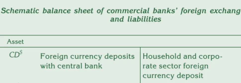
Using the schematic balance sheet drawn up for commercial banks’
foreign exchange assets and liabilities, we are able to express com- mercial banks’ on-balance sheet open positions on the basis of their foreign borrowings, foreign currency deposits with the central bank and foreign currency lending by the central bank as well as foreign currency deposits placed with them.
Table H Schematic balance sheet of commercial banks’ foreign exchange assets
and liabilities
Asset Liability
CD$ Foreign currency deposits
with central bank Household and corpo- rate sector foreign currency deposit
D$
DL$BV Foreign currency lending
to corporate sector Net foreign borrowing of commercial banks
L$FB
OP On-balance sheet open position
Changes in commer- cial banks’ open posi- tions play an important role in for- eign exchange mar- ket intervention
Commercial banks’ on-balance sheet open position shows the surplus of foreign exchange liabilities in the balance sheet over and above foreign exchange assets. Accordingly, ifOP>0, that is, if the value of commercial banks’ foreign exchange liabilities exceeds that of their foreign exchange assets, the balance sheet is characterised by a short position in foreign exchange, or, in other words, a long fo- rint position. Conversely, if OP<0, then foreign exchange assets show a surplus over foreign exchange liabilities, indicating a short forint position.
The change in on-balance sheet open positions can be ex- pressed from Table H using the following equation:
DOP =DD$+DLFB$ –DCD$–DL$BV (8) If DOP>0, resulting in a shift towards a long forint position, commercial banks enter the market with a demand for forint funds, while in the opposite case they appear as suppliers of forint funds, resulting in a shift towards a long foreign exchange position.
Table I shows changes in commercial banks’ balance sheet items as expressed by equation (8). Taking into account the value of financial derivatives, commercial banks’ total open position can be calculated as the sum of their on-balance sheet open position and net foreign currency claims from financial derivatives.
Table I Changes in commercial banks’ open positions (1998, 1999 and 2000 H1)
millions Variables 1998 1999 2000
H1
I Assets (1+2) 740 –249 274
1 Claims on NBH DCD$ 404 –818 –427
2 Foreign currency lending
to enterprises DL$BV 336 568 701
II Liabilities (3+4+5) –152 –532 471
3 Net foreign liabilities DLFB 311 299 715
4 Corporate and household sector
foreign currency deposit DD$ 18 –47 –9
5 Net other liabilities –481 –784 –235
III On-balance sheet open position
(long forint: II– I) DOP –892 –283 197
6 Net foreign currency claims from
derivatives 781 231 –128
IV Total open position
(long forint: III+6) –111 –52 69
3.3.2 Changes in the central bank’s foreign exchange position
Conversion is a broader category than intervention
The total amount of foreign currency converted by the central bank into forint is called conversion. This includes the net forint demand of both the private and the general government sectors. Here, the forint demand of the private sector is exactly equal to the value of foreign exchange market intervention. Forint demand of the general government sector is comprised of the items of the current and cap- ital accounts and a few other items linked to general government (CAG+KAG), foreign currency revenues from privatisation (PvF) and net foreign currency borrowings of the general government sector.
Later, privatisation revenue is divided into two categories, such that can be categorised into foreign direct investments and such that can be classified into foreign currency proceeds from privatisation (PvF
=PvFFDI+PvFE).13Net foreign currency borrowings also include for- eign currency borrowing transactions between general government and the NBH. In practice, this item is primarily the balance of foreign currency borrowings of the central government abroad (DLFK) and repayments of foreign currency lending to the NBH (DLJK). Thus, using the earlier variables, the items comprising conversion are the following:
conversion = Int + CAG+ KAG+ PvF+DLFK+DL$JK
However, conversion is also recorded in the central bank’s bal- ance sheet and is equal to the change in the central banks’ net for- eign exchange assets after elimination of the effects of movements in exchange rates. Table J contains the major foreign currency- denominated items of the central bank balance sheet.
On the basis of the central bank balance sheet, the major items of the change in net foreign exchange assets are the increase in in-
13The balance-of-payments categorisation depends on whether the given non-resident investor has acquired a stake of more than 10 per cent in the company in question. Acquisitions of more than 10 per cent in companies are recorded on the foreign direct investment row of the table.
14This item includes the special foreign currency deposit of the central government with the NBH.
Table J Schematic balance sheet of the central bank’s foreign currency assets
and liabilities
Asset Liability
Res International reserves Foreign currency deposits
of commercial banks CD$ LJK$ Net foreign currency lending
to central government14 Foreign borrowings
of central bank LFJ