A Multi-Variable LQG Controller-based Robust Control Strategy Applied to an Advanced Static VAR Compensator
Ali Tahri, Houari Merabet Boulouiha, Ahmed Allali and Tahri Fatima
Electrical Engineering Faculty, Electrotechnics Department, Laboratory of Electrical Engineering of Oran,
University of Sciences and Technology of Oran USTOMB, BP 1505 El Mnaouar 31000 Oran, ALGERIA
E-mail: ali.tahri@univ-usto.dz, houari.merabet@univ-usto.dz, ahmed.allali@univ- usto.dz, fatima.tahri@univ-usto.dz
Abstract: In this paper, an Advanced Static VAR Compensator (ASVC) based on a voltage type inverter is presented and analysed. The ASVC, which uses the Pulse Width Modulation (PWM) technique, will be modelled in the Park system. Moreover, a low pass filter is introduced at the output of the inverter in order to eliminate the high order harmonics. The proposed system may compensate inductive or capacitive reactive power. The mathematical model thus obtained will be used for the design of a linear quadratic Gaussian (LQG) multivariable (MIMO: Multiple Input Multiple Output) control strategy.
The simulation results obtained with MATLAB software are included and will be thoroughly discussed in this paper.
Keywords: LQG controller; multi-variable control; VAR; Programmed PWM; Low pass filter; ASVC; Matlab; Simulink; SimPowerSystems toolbox
1 Introduction
Reactive power is known to be responsible for frequency changes in the voltage of the network and a weakening of the power factor.
The increase in the absorption of this reactive energy creates disturbances on the transmission line.
In an ideal AC system, the voltage at each nodal point should be constant and free of harmonics, with a power factor close to unity; however these parameters must be independent of the size and characteristics of the load of the consumers. This
can only be guaranteed if the loads are equipped with a means of reactive power compensation, and it is a must that this has very fast dynamic compensation.
Various classical reactive power compensators have been in use for years, particularly those based on thyristors, such as TCR, TSC and SVC.
The TCR compensator (Thyristor Controlled Reactor) is composed of an inductance connected with a Dual switch made up of two thyristors in antiparallel.
Each thyristor is controlled every half cycle. The control of the reactance depends on the load demand by varying the instant of the switching of thyristors [1]. The circulating current in the TCR is thus highly inductive due to the presence of the reactance; i.e. the compensator can only absorb the reactive power [2] – [6].
The TSC Compensators (Thyristor Switched Reactor) are generally composed of dual thyristors, each of which controls a capacitor bank. With the presence of capacitors, the current always leads the voltage, which will undoubtedly result in a flow of reactive power to the network [7].
The combination of TCR and TSC devices result in a hybrid compensator called an SVC (Static Var Compensator), playing on the thyristor firing instant to obtain an equivalent of a continuously variable reactive power source [2] [8] [9].
However, this type of compensators exhibits a major drawback, that of being a source of harmonics [6].
Taking advantage of advances in the field of power electronics, devices of self- commutation have been adopted, such as the Advanced Static Var Compensator (ASVC), which is based on a voltage source inverter. This compensator is very flexible to any fluctuation or changes of the loads; it can either deliver or absorb reactive power instantaneously to improve the stability and dynamic performances of the grid network.
The signals from the states of the switches of the three-phase inverter are obtained through the use of a programmed PWM technique. To improve the quality of energy, we have added a resonant filter based on a low pass filter RLC.
The synthesis of the controller LQG (Linear Quadratic Gaussian) multi-variable is based on a mathematical model of multi-state variable of the ASVC for simultaneously controlling the voltage in the DC side and the reactive power.
The control strategy applied to this type of compensator will be validated by simulation results using MATLAB software
2 Main Circuit Configuration of the ASVC
The proposed circuit of the ASVC (Advanced Static Var Compensator) using a
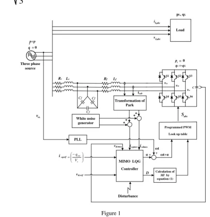
Figure 1 shows the different blocks comprising the circuit configuration of the multi-variable control system of the ASVC compensator. Measurements of the currents of Park in both d and q axes and the DC voltage will be added to a white noise (this noise is generated by a white noise generator).
Fluctuations in the DC side voltage and the reactive power may be possible because of the multi-variable controller, where the output could provide two outputs. The first output is the phase α which is added to ωt. The second output is the conversion ratio between the inverter fundamental output voltage and input DC voltage (D). With the latter, we can calculate the modulation index (MI) by the following equation:
2
MI 3 D
(1)Three phase source
p=p q
S1 S2 S3
S4 S5 S6
C vca
vcb
vcc
Load
s s=0
qc=-qL
Sabc ,
vLabc , iLabc
Ls Rs
icab
,
vsa
c 0 p=
pL, qL
MIMO LQG Controller PLL
vdcmes icqmesicdmes ωt cqréf
i
s ref
V q
vdcréf
α + +
D ωt+α
Calculation of MI by equation (1)
Programmed PWM Look up table Transformation of
Park ++ ++
Disturbance White noise
generator Rf Lf
Cf
Cf Cf
Figure 1
Multi-variable control of the ASVC
3 Programmed PWM
3.1 The Main Objectives of a PWM
We obtain load currents whose waveform is close to a sine wave by controlling the evolution of the duty cycles and thanks to a high switching frequency of the devices with respect to frequency of the output voltages.
To allow fine control of the amplitude of the fundamental output voltages generally to a large extent and for a widely variable output frequency.
3.2 Generation of the Programmed PWM Look Up Table
This PWM technique is used to calculate the switching instants of the devices so as to match certain criteria on the frequency spectrum of the resulting wave. These sequences are then stored and used cyclically to ensure the control of the switches.
The criteria commonly used are:
Elimination of harmonics of a certain range.
Elimination of harmonics in a specified frequency band.
In this paper, we have used the tools of Matlab/ Simulink in order to implement this programmed PWM [10] technique for generating control signals for switches as there is not any block in the SimPowerSystems toolbox.
The modulation index is varied from 0 to 1.15 in steps of 0.01 (that is to say 115 is the value of the modulation index). Each modulation index is shown in a table of ωt for a period of 0.02 sec with a sampling time of 0.02/4096.
The solutions obtained by the Newton-Raphson method to eliminate 10 harmonics for each modulation index is stored in an array of size 4 Kbytes (4 × 1024 = 4096), that is to say 4096 points per cycle.
Then, two counters were designed (one horizontally to detect the modulation index and the other vertically to detect the instant ωt + α and to count from that instant for a period of 0.02 sec in steps of 0.02 / 4096), where the first counter pointer detects the modulation index (MI). Once the modulation index is detected, the pointer of the second counter is attached to the table for the modulation index obtained by the first counter from the time ωt + α, as shown in Figure 2.
SA
MI
SA SB SC
SA SB SC
0.01
MI
SB
SC
Programmed PWM Look up Table wt+
Figure 2
Programmed PWM look-up table generation method
A low pass filter is added to the output of the voltage type inverter in order to eliminate high order harmonics produced by the inverter and which are not eliminated by the programmed PWM.
Figure 3 shows how the programmed PWM is implemented in Matlab/Simulink. It is composed of two major parts, the first part is the counter which itself is made of two counters, one horizontal to detect the modulation index and the other vertical to detect the instant ωt + α, the second part is the PMW look up table.
Figure 4 shows the details of the counter block, where an Mfile was developed and implemented as a MATLAB function.
Finally, Figure 5 shows the generation of the programmed PWM block diagrams where three 2 dimensional direct look up tables SIMULINK blocks are used, each for one phase.
Figure 3
Programmed PWM block in MATLAB/SIMULINK
Figure 4
Counter Bloc in MATLAB/SIMULINK
Figure 5
Inverter Pulses Generating Bloc in MATLAB/SIMULINK
4 Modelling and Analysis of the ASVC System
Functions of the Pulses are given by the following equation:
sin sin 2
3 sin 2
3
a b c
S t
S S MI t
S
t
w +
w w + + +
(2)
The mathematical model of the ASVC currents in the axes of Park (d-q) is:
sin cos
s s s cq s
s s s cd s dc
L p R L i V
L L p R i V Dv
+ w
w +
(3) Where,V
s : is the effective value of the source voltage.D: is the conversion ratio of the inverter between the fundamental of the output voltage and the DC input current. α: is the phase angle between the network voltage and the output voltages of the inverter.
p: Laplace Operator.
The equation in the DC side in d-q is given by:
dc
cd s
dv D
dt C i
(4) After manipulation, we find the system state multivariable of the ASVC in Park [7], [11]:
1
x t Ax t Bu t y C x t
+ +
(5) With:0
0
0 1 0 0
, 1 0 ,
0 0 1
0 0
0 0
s s
s s
dc
s s s
s
R
L V
R D
A B v C
L L L
D C
w
w
cq cd dc
,
x i i i
u D
Where:
A is the state matrix, B is the input matrix, C is the output matrix, x is the state vector, u is the input vector and y is the output vector.
5 Synthesis of the Controller LQG MIMO
The control method LQG consists of an LQR (Linear Quadratic Regulator) with the observer states of the system via the method of the Kalman filter. In the case where the system state (5) is a linear one or linear around an operating point, we can represent it as in the following form:
1
x t Ax t Bu t M w t y C x t v t
+ + +
+
(6)With:
10.124 7.33 2.31 5.12 10.555 20.66 M
Where w(t) and v(t) represent white noise with zero as mean value, independent, respectively, with covariance matrix W and V.
122
2
9
100
E w t w
Tt W t
1
1
E v t v
Tt V t
Where:
E : mathematical esperance.
δ : is the Kronecker Symbol.
The Kalman filter matrices are supposed to be symetrical:
T
0
f f
Q Q
andR
f R
Tf 0
(7) Where such weighting matrices are given by:T f
f
Q MW M
R V
(8) With:2
9 0 0 100 W
V I
(9)
The estimating gain Ke of Kalman is obtained by the following relation:
T 1e f
K t P t C R
(10) Where Pf is the solution matrix of Riccati equation:1
0
f f f f f f
P A + A P
P BR B P
+ Q
(11) The synthesis of the LQR controller consists then in finding a matrix with gain L and where the optimal feedback control is given by [12]:
u
opt Lx t
(12) The minimizing quadratic criterion for obtaining the control law (12) is:
0
J
LQRx Qx u Ru
+
(13) Where the weighting matrices Q and R are given by:2
Q C C R I
(14) Where:I2: is the identity matrix of dimension 2.
The necessary condition for optimum of the derivative being zero of the cost function J LQR leads to the solution:
L R B P
1 (15) Where P obeys the algebraic equation of Riccati [13]:P PA A P PBR B P Q
1
+
(16)Considering the steady state solution of this equation P, which is done in most cases in the literature, it is sufficient to solve the following equation:
1
0
PA + A P
PBR B P Q
+
(17) Figure 6 shows the schematic diagram of the LQG control method, where the term N is calculated in steady state to eliminate the static error by the following equation [14]:
1 1N C I A BL B
+
(18)Figure 6
The structure of LQG Controller
r C
A S-1I System + + +
-
u x y
Ke
B S-1I C
A
L
++ + + -
e(k+1)
Estimator
N B
6 System Blocs Design in Matlab/Simulink
The proposed system is composed of two main parts: one consists of the control circuit and the second part is concerned with the power side.
The bloc representing the controller (control section) MIMO LQG in Matlab Simulink is shown in Figure 7.
Figure 7
Detailed Circuit Diagram of the LQG MIMO
The simulation model of the ASVC is implemented in Matlab / Simulink as shown in Figure 8 using SimPowerSystems toolbox blocs. However, the ASVC is implemented by the universal bridge block with IGBT switches. In order to synchronize the ASVC with the supply a discrete three phase PLL is used.
In order to simulate the ASVC operating from 10KVARcapacitive to 10KVARinductive two 3 phase RLC parallel loads are used and switched on and off with two 3 phase breaker blocks.
To run the simulation quickly, a discrete mode is chosen in powergui block, which is the environment block for SimPowerSystems models. The sample time for the simulation is set to the same sampling time (0.02 / 4096) as calculated for the PWM look up table as given in section 3.2.
Figure 8
Block Kalman filter in MATLAB / SIMULINK is shown in the following figure:
Figure 9
Detailed Circuit Diagram of the Kalman filter
7 RLC Filter Synthesis
A low pass filter has been chosen to eliminate the high order harmonics produced by the inverter which are not eliminated by the programmed PWM technique, where the capacitors of the filter are Delta connected. The transfer function of the filter is given by:
2 0
2
0 0
1
1 2 2
f
f f f f
G j
L C j R C
w
w w w
w + w
(19)
Where:
ω: is the pulsating frequency.
ωo: is the particular pulsating frequency.
This function has a dynamic of the second order. By identifying the denominator to the canonical form as follows:
0 0
2 1
j w w
+ +
w w
(20) After calculation we find:0
1 2
2
f f
f f
f
L C R C
L
w
(21)
With:
ξ: is the damping coefficient.
By fixing Rf =1Ω, ωo=6×ωs (where ωs=2×π×50) and ξ=0.083. After calculation we obtain:
0
2 0
2 3.2
1 43
2
f f
f
f
L R mH
C F
L
w
w
We choose the commercially available value, thus the values of the filter are:
f
3.3
L mH
andC
f 40 F
8 Simulation Results
The simulation results are obtained by using the following parameters:
Network :
3.4 , 3.3
s s
R L mH 380 , 50 V
s V f Hz
DC side:
s
500 C F
0.8 3 , 800 D 2 v V
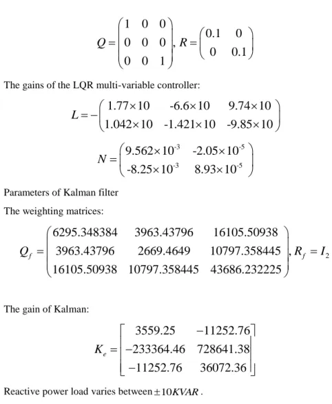
Parameters of the LQR MIMO controller:
1 0 0
0.1 0 0 0 0 ,
0 0.1 0 0 1
Q R
The gains of the LQR multi-variable controller:
1.77 10 -6.6 10 9.74 10 1.042 10 -1.421 10 -9.85 10
L
-3 -5
-3 -5
9.562 10 -2.05 10 -8.25 10 8.93 10
N
Parameters of Kalman filter The weighting matrices:
2
6295.348384 3963.43796 16105.50938 3963.43796 2669.4649 10797.358445 , 16105.50938 10797.358445 43686.232225
f f
Q R I
The gain of Kalman:
3559.25 11252.76 233364.46 728641.38 11252.76 36072.36 K
e
Reactive power load varies between10KVAR.
Figure 10 shows the waveforms of the load current iLa, the compensator current ica and that of the source isa, respectively, with respect to the supply voltage vsa for both inductive and capacitive modes.
At the time of the operation of the compensator at t = 0.02 sec, we notice that the supply current becomes in phase with its voltage. At time t = 0.1 sec, a disturbance was applied to the system states, and we notice that despite the disruption the current isa stays in phase with its voltage vsa. The DC voltage vdc, measured and estimated with its reference and current idc on the DC side as well as the shape of the supply and compensator voltages and the modulation index MI, are illustrated in Figure 11. Moreover, we noticed that the DC side voltage follows perfectly its reference of 800V before and after the disturbance.
Figure10
Waveforms of the source voltage, respectively, with the load, compensator, and source currents
Figure11
Responses of the DC side voltage and current with network and compensator voltage and modulation index MI for vdcref=800V
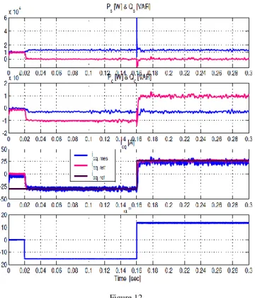
Figure 12 shows from top to bottom the active and reactive power at supply bus bar. We notice that the ASVC from t=0.02 sec to 0.16 sec generates 10KVARcapacitive reactive power to compensate for the inductive reactive power absorbed by the load, and from 0.16 sec it absorbs the reactive power generated by the capacitive load.
The estimated and measured reactive currents both follow the reference of the reactive current. Finally, the phase angle α between the network voltage and the output voltages of the inverter is depicted; it is clear that when the ASVC is in capacitive mode α is negative and when the ASVC is in inductive mode it is positive.
Figure 12
Responses of the active and reactive power respectively of the network and compensator, and the reactive component of the current of the compensator, and control law α
Conclusions
In this paper, an Advanced Static Var Compensator (ASVC) using a voltage type inverter has been thoroughly discussed.
The LQG controller (Linear Quadratic Gaussian) is composed of a regulator, LQR MIMO (Multi Input Multi Output), with an observer of the system states through a Kalman estimator.
The synthesis of the MIMO LQR controller is based on a mathematical model of the multi-variable state of the static reactive power compensator in the dq axes of Park. The synthesis of the Kalman filter is based on the perturbation matrix (M) and by white noise chosen by the manufacturer.
This control strategy exhibits better speed and good filtering of the white noise, with the possibility of controlling simultaneously the reactive component of the compensator current icq and the DC side voltage vdc..
The switching signals from the semiconductor devices of the three-phase inverter are obtained through the use of a programmed PWM technique.
References
[1] E. Acha, V. Agelidis, O. Anaya, TJE Miller, “Power Electronic Control in Electrical Systems”, Newnes, 2002
[2] S. Khalid, N. Vyas, “Applications of Power Electronics in Power System”, Laxmi Publications Pvt limited, 2009
[3] G. W. E. Moon, “Predictive Current Control of Distribution Static Compensator for Reactive Power Compensation”, IEEE Proc-Gener.
Tunsm. Distrib, Vol. I46, No5,September 1999
[4] E. Acha, C. R. Fuerte-Esquirel, H. Ambriz-Perez, C. Angeles. Camacho,
“FACTS Modelling and Simulation in Power Networks”, John Wiley and Sons, Ltd. 1004
[5] N. Mohan, T. M. Undeland, W. P. Robbins “Power Electronics, Converters, Application, and Design”, Second Edition, John Wiley and Sons, Inc. 1989 [6] Fatima Tahri, “Contribution à la commande d’un compensateur statique
d’énergie réactive”, Thèse de Magister, USTO, 11 Juillet 2006
[7] Houari Merabet Boulouiha, “Commande adaptative d’un compensateur statique de puissance réactive », Thèse de Magister, USTO, 17 Juin 2009 [8] V. K. Sood, “HVDC and FACTS Controllers Applications of Static
Converters in Power Systems”, Kluwer Academic Publishers, Boston. 2004 [9] A. Tahri, “Analyse et Développement d’un Compensateur Statique Avancé Pour L’amélioration de la Stabilité transitoire des systèmes Electro- Energétiques”, Thèse de Magister, USTO, Juillet 1999
[10] SimPowerSystems User’s Guide, the Mathworks Inc 1990
[11] Guk C. Cho, Gu H. Jung, Nam S. Cho and Gyu H. Cho, “Control of Static VAR Compensator (SVC) With DC Voltage Regulation and Fast Dynamique By Feedforward and Feedback loop”, Conférence IEEE Conf.
Pub, 367-374 Vol. 1, 26th annual meeting, pp. 7803-2730-6, Korea, 18-22 Jun 1995
[12] André. Noth, “Synthèse et Implémentation d’un Controleur pour Micro Hélicoptère à 4 Rotors”, Ecole Polytechnique Fédérale de Lausanne, Institut d’Ingénierie des Systèmes, I2S Autonomous Systems Lab, ASL, Février 2004
[13] Daniel. Alazard, “Régulation LQ/LQG, Notes de cours”
[14] Houari. Merabet Boulouiha, Ali. Tahri et Ahmed. Allali “Commande Multi-Variable d’un Compensateur Statique de Puissance Réactive Par L’utilisation d’un Régulateur Linéaire Quadratique LQR”, 2èmes Journées Internationales d’Electrotechnique, de Maintenance et de Compatibilité Electromagnétique à l’ENSET Oran, Conférence Internationale JIEMCEM’
2010,25-27 Mai 2010