(will be inserted by the editor)
Analysis of the tyre-road interaction with a non-smooth delayed contact model
S´andor Beregi · D´enes Tak´acs
Received: date / Accepted: date
Abstract In this study a tyre model is developed for multibody dynamics soft- ware. Vibrations of a towed wheel excited by the lateral deformation of the tyre are analysed with the help of numerical simulations. In our calculations the time delay in the tyre-ground contact as well as the partial side slip are considered making it possible to capture the dynamic deformation of the contact patch centre-line with relatively low number of parameters and computation time. As a result the hysteresis effect in the stability of the rectilinear motion can be identified, which would be undetectable by simpler, quasi steady-state tyre models. Thus, bistable parameter regions appear in the stability charts where for the same set of system parameters a stable equilibrium and a periodic orbit coexist. The simulations are compared with measurements carried out on an experimental rig consisting of a wheel and a caster running on a conveyor belt.
Keywords tyre-road contact·dynamic tyre·deformation·non-smooth delayed tyre model·lateral vibrations·wheel shimmy
ACKNOWLEDGEMENT
This research has been supported by the ´UNKP-17-13-I. New National Excellence Program of the Ministry of Human Capacities.
S. Beregi
Department of Applied Mechanics, Budapest University of Technology and Economics, Bu- dapest, Hungary
H-1111, Budapest, M˝uegyetem rakpart 3.
Tel: +36 1 4631235 E-mail: beregi@mm.bme.hu D. Tak´acs
MTA-BME Research Group on Dynamics of Machines and Vehicles, Budapest, Hungary H-1111, Budapest, M˝uegyetem rakpart 3.
E-mail: takacs@mm.bme.hu
1 Introduction
The contact between different bodies is often the most challenging task in designing multibody dynamics software. Amongst many other applications these kind of software are widely used by car manufacturers for simulating the behaviour of the entire vehicle or certain parts of it in a hardware-in-the-loop environment. In analyses focusing on vehicle handling it is essential to use a realistic model of the contact forces developing as the tyres deform interacting with the road-surface while the vehicle is moving and the tyres are rotating. The instantaneous shape of the tyre is influenced by past and present states of the vehicle, which induces a memory effect in the contact. Moreover due to the contact friction the phenomenon of force-generation is highly non-smooth and nonlinear as well, therefore it often requires complex algorithms to implement all the relevant effects into the tyre model. On the other hand there is a demand to carry out these calculations as quickly as possible which eventually leads to a compromise between accuracy and computation time.
Several tyre models have been developed to capture the deformed shape of the contact region and calculate the resulting tyre forces. The most commonly used models are assuming quasi-steady state deformation in the contact region, making it possible to introduce tyre force and aligning moment characteristics, which can be well used for analysis at larger vehicle speeds [1, 2]. However, for low or medium velocities these models tend to be inaccurate as the memory-effect associated to the time-delay becomes more relevant in the contact [3, 4]. One solution to overcome this issue is to use additional degrees of freedom addressed to certain dynamic features of the tyre together with the tyre force characteristics [5]. For example the models MF-SWIFT [6] and FTire [7] are both take into account the elasticity of the tyre belt and carcass beside the contact forces, making them capable to capture vibrations up until∼80-150 Hz. These models can be effectively used in multibody simulation algorithms; nevertheless, due to the higher number of parameters one may find these less convenient for a qualitative analysis of tyre dynamics. Another solution is to use continuum-based tyre models which are capable to describe the travelling waves in the rolling tyre-ground contact. Unfortunately these lead to partial differential equations, which can be solved only numerically, e.g. using finite element algorithms [8, 9, 10], which can be computationally very costly.
We selected the stretched string tyre model [1] for our studies, which can be a good compromise in this respect since for pure rolling the deformation is described by a single PDE. This model also takes into account the tyre deformation outside the contact-patch, which has a relevant effect in the low velocity-range [3]. For the nonlinear PDE a travelling wave solution can be composed analytically by introducing time delay distributed along the contact length. If the delayed tyre model is implemented in simple vehicle-handling models such as the 3.5 degree- of-freedom single track model of the car-trailer combination, then beside the well- known unstable parameter domains at large velocity a rich structure of alternating stable and unstable parameter regions at low speed is revealed. Such a structure of parameter domains appears if a similar model of a standalone car is investigated [4] and even the stability chart of the straight-line motion of a single towed wheel shows similar features [3]. This motivated us to concentrate on the analysis and development of the contact model by means of a simple vehicle model keeping in
mind that in later studies the improved tyre model may be implemented in more complex multibody system models.
In spite of its effectiveness in linear stability analysis the travelling wave so- lution cannot capture the sliding effect caused by friction in the contact region.
Thus, to investigate the nonlinear dynamics it has to be enhanced by taking into account the side slip, too.
Considering the memory effect and the contact friction simultaneously in the tyre-road contact can result a complex structure of sticking and sliding regions, as for the stretched-string model in particular, the deformation in the sliding parts is described by differential equations [11]. It is worth to mention that in contact mechanics several studies revealed a similar structure of sticking and sliding re- gions in the frictional contact of elastic continua [12]. In our study we introduce a case-selective algorithm to determine the boundaries and the deformation in the different regions that can occur while the tyre makes lateral vibrations. Then the non-smooth delayed tyre model is implemented in the numerical simulation of a towed wheel. By obtaining the stable periodic solutions in the system we demonstrate the hysteresis effect observed in practice regarding the stability of the rectilinear motion.
2 The governing equations of a shimmying wheel
dt
V
X Y
x y
ψ(t) q(x,t)
T
A
l JA F
M
deformed tyre centre-line
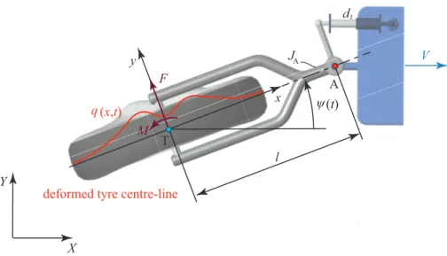
Fig. 1 The in-plane model of a towed wheel with a rigid caster.
In this study we implement our tyre model into the in-plane model of a towed wheel (see Fig. 1) attached to a rigid caster of length l, which is towed by a constant velocity V along the X-direction. The whole system has a mass of m
and a mass moment of inertia JA with respect to the joint A. One can use the deflection angle ψ(t) as a generalised coordinate to describe the position of the system in the (X, Y) coordinate-plane. To the king pin A a torsional damper with a damping coefficient ofdt is attached.
Using Lagrange’s equation of the second kind, one can derive the equation of motion of the yaw vibrations of the wheel as
JAψ¨(t) +dtψ˙(t) =M−F l, (1) whereF andM are the lateral contact force and aligning torque generated by tyre deformation, while dots refer to time-derivatives.
3 The non-smooth delayed model of the tyre-ground contact 3.1 The stretched-string tyre model
y
x q(x,t)
p(x,t)
-a a a+σ
-a-σ
k d,
P L
R
material flow direction
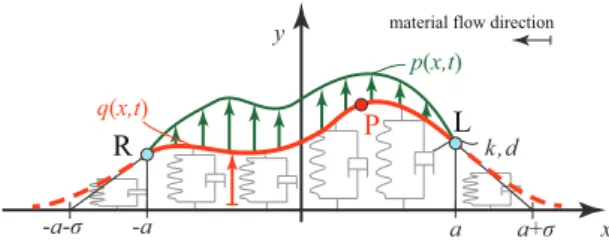
Fig. 2 The stretched string tyre model with the distributed lateral forcep(x, t) in the contact patch and relaxation (dashed curves) outside the contact region.
The tyre forces are calculated via the stretched-string tyre model [1, 13], by means of which the elastic tread and carcass of the tyre is modelled as a stretched string supported by linearly distributed spring and damper elements with stiffness and damping parameters of k and d. It is assumed that tyre damping is large enough not to allow deformation waves travelling around the wheel to have sig- nificant interference between the deformations of the leading (x=a) and trailing (x=−a) edges. Thus, an in-plane model with a stretched string of infinite length shown in Fig. 2 is used. In thex∈[−a, a] contact patch a distributed force system ofp(x, t) is applied to the string resulting in the deformation of the tyre, whereas outside the contact patch the tyre is assumed to be unloaded in the lateral direc- tion. With the consideration above the lateral deformation of the string can be described by the following PDE:
kσ2q′′(x, t)−dq˙(x, t)−kq(x, t) =p(x, t), (2) whereq(x, t) is the lateral deformation of the string,σis the tyre relaxation length while primes refer to derivatives with respect to coordinatex.
Then, according to the classical stretched string model [1, 13] the resultant tyre forces are calculated by integral formulae
F =k
∫∞
−∞
q(x, t) dx+d
∫∞
−∞
d
dtq(x, t) dx (3)
and
M =k
∫∞
−∞
x q(x, t) dx+d
∫∞
−∞
x d
dtq(x, t) dx . (4) 3.1.1 Deformation in the contact patch in case of pure rolling
In case of pure rolling (no side-slip considered) the tyre is assumed to stick to the ground and the tyre centre-line to have zero relative velocity in the x ∈[−a, a]
contact patch. This can be formulated as a kinematic constraint as d
dtRP= 0, (5)
whereRPis the position vector of an arbitrary point P of the contact patch centre- line in the ground-fixed frame of reference. Based on this, a nonlinear PDE can be derived which describes the lateral deformation in the contact patch
˙
q(x, t) =V sinψ(t) + (l−x) ˙ψ(t)−q′(x, t) (
q(x, t) ˙ψ(t)−Vcosψ(t) )
. (6) For this equation a so-called travelling wave solution can be composed, which yields to a formula with a time delay ofτ(x) distributed along the contact region
q(x(τ), t) =V τsinψ(t)−(a−l) sin (ψ(t)−ψ(t−τ))
+q(a, t−τ) cos (ψ(t)−ψ(t−τ)) (7) while the longitudinal distribution of the time delayτ(x) can also be expressed.
Thus, for the coordinatexwe get
x(τ) =−V τcosψ(t)l+ (a−l) cos (ψ(t)−ψ(t−τ))
+q(a, t−τ) sin (ψ(t)−ψ(t−τ)). (8) Due to the rolling of the tyre it is reasonable to assume that no kink (discon- tinuity in the first derivatives) in the deformed shape arises at the leading edge (x=a), where the tyre particles first touch the ground. This can be formulated in the following boundary condition
q′(a, t) =−q(a, t)
σ . (9)
Applying this we can compose an ODE for the lateral deformation at the leading edge
˙
q(a, t) =Vsinψ(t)−(a−l) ˙ψ(t) +q(a, t) σ
(
q(a, t) ˙ψ(t)−V cosψ(t) )
. (10) Note, that discontinuity in the first derivatives cannot show up at the trailing edge R either as it would result a dirac-delta like peak in the distributed lateral load. However as the PDE is first order in coordinate x exactly one boundary condition can be attached to it. Hence, the ‘no kink’ condition at the trailing edge is considered by handling sliding.
3.1.2 Partial side-slip in the contact patch
x y
a x x
-a R L
qr(x,t) qsL(x,t) qsR(x,t)
qrel(x,t) qrel(x,t)
rolling sliding
tyre sl.
relaxation
tyre relaxation
Fig. 3 The different contact regions assumed. The rolling region is white while the sliding regions are shaded. The continuous line corresponds to tyre parts in contact with the ground while the dashed lines to the tyre relaxation regions.
If the effect of dry friction in the tyre-ground contact is considered, the con- dition of rolling holds only limitedly as side-slip will occur in those parts of the contact region where the intensity of the distributed force system corresponding to rolling is larger than the limits determined by friction. We assume a parabolic normal force distribution along the contact length. Although one may experience a shift in the vertical load towards the leading edge for large velocity, moreover, a non-parabolic distribution is also very common for larger contact patches,this is an acceptable simplification for the low and medium speed-ranges which are in the focus of our analysis. By means of this assumption the lateral force limits are also defined by parabolae [1] as
pr+(x) = 3Fzµr
4a3 (
a2−x2 )
, pr−(x) =−3Fzµr
4a3 (
a2−x2 )
,
(11)
and
ps+(x) = 3Fzµs
4a3 (
a2−x2 )
, ps−(x) =−3Fzµs
4a3 (
a2−x2 )
,
(12)
whereprr+andpr−are the distributed lateral force limits corresponding to rolling, ps+ and ps− are the limits corresponding to sliding. Fz is the vertical load of the tyre whereas µr and µs are the friction coefficients for rolling and sliding, respectively. It follows from the above that for the rolling part of the contact patchp(x)∈[pr−(x), pr+(x)] should hold.
The limits for sliding give the distributed force system for the sliding parts of the contact patch in question. Therefore, we can substitute these into Eqn. (2) to calculate the deformation in these zones. Unfortunately, this PDE is badly- conditioned in terms of the required time-step for numerical simulation, which would slow down our computation. Therefore, in the sliding regions we use the
steady-state solutions q(x, t) = qs(x, t), ˙q(x, t) ≡ 0 of Eqn. (2) which can be calculated from the following ODE
qs′′(x, t)−qs(x, t)
σ2 =± 3Fzµs
4a3kσ2 (
x2−a2 )
(13) where the sign of the right-hand side depends on the sliding direction. For this differential equation the analytical solution can be provided as
qs(x, t) =C1exσ +C2e−xσ± 3Fzµs
4a3k (
a2−x2−2σ2 )
, (14)
where the constantsC1andC2can be calculated from the corresponding boundary conditions, which are to be discussed later on.
3.1.3 Deformation outside the contact patch
The deformationqrel(x, t) outside the contact patch can be calculated in a similar way as for the sliding parts assuming a quasi-stationary deformation asq(x, t) = qrel(x, t), ˙q(x, t)≡0. Since we assume no lateral load in this region Eqn. (2) yields to a homogeneous differential equation
q′′rel(x, t)− qrel(x, t)
σ2 = 0. (15)
Using the boundary conditions qrel(a, t) =qsL(a, t), limx→∞qrel(x, t) = 0 and qrel(−a, t) =qsR(−a, t), limx→−∞qrel(x, t) = 0 the deformation can be expressed as
qrel(x, t) =qsR(−a, t)ea+xσ forx∈(−∞,−a], (16) and
qrel(x, t) =qsL(a, t)ea−xσ forx∈[a,∞). (17) 3.1.4 Boundary conditions at the sliding regions
For the case of simplicity in this study we only consider those cases, when sliding regions occur both at the leading edge and at the rear end of the contact patch and the whole contact patch slides only when the sliding regions merge. It can be shown that this assumption can be used for the analysis of wheel-shimmy. Fig. 3 shows the assumed structure of the different types of regions in the contact. Thus, in general we consider three different regions in the contact patch: a sliding region at the leading edge (x∈[xL, a]), a rolling region in the middle (x∈[xR, xL]) and a sliding region at the rear edge (x∈[−a, xR]). In the rolling part the deformation is described by the travelling-wave solution (see Eqn. (7)), whereas in the sliding parts the ODE (13) applies.
To provide a sufficiently smooth transition between the different regions of the contact patch, on one hand, the conditions of continuity should hold for the boundaries
qr(xL, t) =qsL(xL, t). (18) qsR(xR, t) =qr(xR, t). (19) Studying the PDE of Eqn. (2) it can be also shown that the first derivatives with respect to the coordinatexshould be continuous as well. This is due to the fact,
that a discontinuity would involve a dirac-delta like ‘peak’ in the lateral force distribution, which would be incompatible with the lateral distributed force limits (11). Thus
q′r(xL, t) =q′sL(xL, t), (20) qsR′ (xR, t) =q′r(xR, t). (21) Based on the same principle, another two boundary conditions can be formu- lated for the leading and rear edges which are equivalent to the ‘no kink’ conditions at the ends of the contact region
qr′(a, t) =−qsL(a, t)
σ , (22)
qsR′ (−a, t) = qr(−a, t)
σ . (23)
These considerations however lead to an over-constrained problem for the slid- ing regions since we formulated three boundary conditions for both the sliding parts at the leading and rear edges, whereas the existence and uniqueness of the solutions of the ODE (13) is assured by attaching two boundary conditions. There- fore, we find the solution by varying the boundaries of the sliding regionsxL and xR, using the boundary conditions of Eqns. (19), (18), (23) and (22) in Eqn. (13), whereas the continuity of the first derivatives (Eqns. (21), (20)) is used to find the boundaries between the rolling and sliding regions.
3.2 Numerical calculation of the deformation
The presented numerical method is constructed such that it can be implemented in a one-step explicit differential equation solver (in our study fourth order Runge- Kutta is used). In each time-step the corresponding deformed shape is calculated in two substeps. Firstly, based on the travelling wave solution we provide the tyre deformation as if the condition of pure rolling would hold for the whole contact patch. Unfortunately, due to the sliding region at the leading edge the travelling wave solution cannot be used as it is given in Eqn. (7) since the tyre particles do not stick at x=ain general. This problem could be handled if we would use the past values of the position and the lateral deformation of the transition from sliding to rolling at the leading edge. However, since the limit is varying in time this should be performed for every single point of the contact region separately.
Instead, it is much more convenient to store the deformed shape of the contact line from the last time-step as it already contains the ‘memory-effect’ in the tyre- ground contact, and calculate the deformation in discrete points using the same incremental time delay stepshin the formula as
q(xi, t) =V hsinψ(t)−(xi−1−l) sin (ψ(t)−ψ(t−h))
+q(xi−1, t−h) cos (ψ(t)−ψ(t−h)), (24) whereas for the longitudinal position of the tyre particles we obtain
xi=−V hcosψ(t)l+ (xi−1−l) cos (ψ(t)−ψ(t−h))
+q(xi−1, t−h) sin (ψ(t)−ψ(t−h)), (25)
where i = 2, ..., N if the contact patch is discretised by N points as a = x1 >
x2 > ... > xN−1 > xN = −a. Meanwhile, the leading point deformationq(x1, t) is obtained from the ODE (10).
Then, the lateral distributed force system required for the calculated deforma- tion is obtained based on Eqn. (13) as
preq(xi, t) =−kσ2q′′(xi, t) +kq(xi, t) (26) where the second derivativeq′′(xi, t) is calculated by finite differences. The lateral force is compared to the limiting parabolae which provides us an initial guess for the two rolling/sliding transition boundaries. Using these we find the location of the transition between rolling and sliding where the continuity of the first deriva- tives holds. If more than one solutions are found, we use the one closest to the initial guess.
This process is straightforward for the sliding region at the leading edge; how- ever, at the rear end sliding can occur either in one or two directions simultane- ously. This phenomenon can be originated in the fact that the continuity of the first derivatives is not assured by the travelling wave solution at the rear end of the contact patch, which would generate another ‘kink’ in the lateral force distribution atx=−a. Since this is incompatible with the lateral force limits it induces sliding at the end of the contact zone. If this sliding happens in the other direction as for the other parts of the rear sliding region, i.e. sgn (preq(−a, t))̸= sgn (preq(x, t)) for x∈(−a, xR) the sliding zone at the rear end is split into two regions with respect to sliding direction. Therefore, for the rear end it should be decided first, whether one or two sliding regions appear, then based on the initial guess the limits of the sliding regions are determined. For sliding in one direction this can be performed straightforwardly, if there are two sliding regions however, this yields to a two di- mensional problem. Thus, we use an additional condition, that the side-change in the resulting distributed lateral force system should be the closest to the position determined based on the travelling wave solution.
4 RESULTS
Before numerical simulations of the nonlinear oscillations of the towed wheel, the linear stability of the rectilinear motion was analysed. In the presented cases the system parameters given in Table 1 were used. The stable and unstable regions regarding the straight-line motion shown in Fig. 4 were determined by studying the governing equations by semi-discretising the PDE in Eqn. (2) describing the lateral deformation.
Running the system in the parameter range where the rectilinear motion is unstable we captured the stable periodic orbits the system converged to. Looking at the the deformed shape of the tyre corresponding to the vibrations of the wheel (see Fig. 5 ) it can be observed that one and two-directional sliding zones alternate at the rear end of the contact patch.
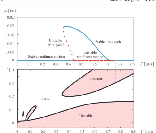
The amplitude of the yaw angleψcorresponding to the stable limit cycles are shown for the caster length ofl= 0.3 m in Fig. 4 compared with the linear stability chart. It was found that there exists a so-called bistable parameter range where despite the fact that the straight-line motion is stable, for large enough perturba- tion the system still can converge to a periodic orbit. From another point of view
0 0.005 0.01 0.015 0.02 0.025
0 0.1 0.2 0.3 0.4 0.5 0.6 0.7 0.8 0.9 V [m/s]
ψ [rad]
Stable limit cycle
Stable rectilinear motion
Unstable rectilinear motion Unstable
limit cycle?
0 0.1 0.2 0.3
l [m]
0 0.1 0.2 0.3 0.4 0.5 0.6 0.7 0.8 0.9 V [m/s]
Unstable Stable
Unstable
Fig. 4 Bifurcation diagram and linear stability chart of the rectilinear motion. In the upper panel blue continuous lines correspond to stable, while red dashed lines to unstable solutions.
In the figure the amplitude ψmax of the deflection angle is shown for different longitudinal velocities. In the lower stability chart, which was constructed in the plane of the towing velocity V and the caster lengthl, the stable and unstable domains are separated by thick black lines.
The white domains are linearly stable, whereas the red shaded regions are linearly unstable.
Parameter Notation Value
Mass moment of inertia with respect to the joint A JA 3.61 kgm2
Tyre-ground contact patch half-length a 0.0395 m
Tyre relaxation length σ 0.13 m
Distributed tyre stiffness k 62600 N/m2
Distributed tyre damping d 19 Ns/m2
Torsional damping at J dt 0.61 Nms
Vertical tyre load Fz 180 N
Friction coefficient for rolling µr 1.5
Friction coefficient for sliding µs 1.0
Table 1 List of parameters used in simulation.
this property of the system can be seen as a hysteresis effect in the stability of the equilibrium. Namely, if the system diverges from the straigth-line motion in the linearly unstable velocity range due to small perturbations, it can be returned to the straight-line motion by decreasing the velocity to a lower value than the linear stability boundary. And similarly, if the perturbations are small by increasing the
-0.1 -5000
5000
-0.01 0.01
0.1
-0.1 0.1
x [m]
x [m]
p [N/m]
-5000 5000
-0.01 0.01
-5000 5000
-0.01 0.01
-5000 5000
-0.01 0.01 q [m]
-0.1 x [m] 0.1
-0.1 x [m] 0.1
-0.1 x [m] 0.1 -0.1 x [m] 0.1
-0.1 x [m] 0.1 -0.1 x [m] 0.1
p [N/m]
q [m]
p [N/m]
q [m]
p [N/m]
q [m]
(a) (b)
(c) (d)
0 t [s] 1
-0.05 0.05 ψ [rad]
(a) (b) (c)
(d)
Fig. 5 The distributed lateral force system and the deformed shape of the tyre centre-line at different time instants. In the top panel the deflection angle is shown while we also marked the four time instants to which the presented tyre deformations and lateral forces correspond.
For each case in the upper panels the continuous and dashed red parabolae represent the force limits for rolling and sliding respectively, while actual lateral load is shown by thick green curves. In the lower panels white zones correspond to the rolling part, red zones to the sliding part (different shades of red refer to two-direction sliding). The regions outside the contact-patch are illustrated by dashed curves.
towing velocity again, the vibrations of the system decay to the stable equilibrium as long as the velocity does not reach the boundary of linear stability.
This feature in dynamical systems can be associated with a subcritical Hopf bi- furcation of the equilibrium corresponding to the straight-line motion. This means that although they cannot be obtained by simulation, at the linear stability bound- ary a branch of unstable limit cycles should emerge above the branch of stable equilibria to separate the ranges of attractivity of the stable equilibrium and the periodic orbit [14]. It is also visible that the branch of the stable limit cycles emerge close to linearly in the plane of the towing velocity V and the amplitude of the deflection angleψmax, which is a typical property in piecewise-smooth differential equations [15].
5 MEASUREMENTS
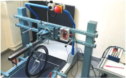
Fig. 6 The experimental rig.
Measurements have been carried out on a towed tyre running on a conveyor belt (see Fig. 6) in order to validate the non-smooth delayed tyre model. In the experimental rig the tyre and the caster are mounted to the ground-fixed rack by a rotational joint while underneath the rubber-made conveyor belt is running with a given speed ofV. With the Galilean transformation this setup can be converted to be identical to the investigated mechanical model.
In the experiment, the wheel is placed into a fork that can be moved along the caster to modify the caster length. The caster can rotate about the vertical axis of the king pin where two preloaded ball bearings are installed in O-type arrangement with oil lubrication. This installation of the bearings leads to a relatively rigid king pin setup having small effect of the dry friction, low damping and no clearance. In the experimental rig, the length of the contact patch can be set by the changing of the vertical distance between the king pin and the conveyor belt. Of course, this construction cannot guarantee constant vertical force acting on the wheel, but none of the experimental results suggested that relevant variation is present for the applied parameter setup.
To reduce the effect of the lateral elasticity of the conveyor belt, it was sup- ported by a rigid frame. Moreover, the tyre inflation pressure and the contact patch size were tuned to smaller values, where preliminary experiments showed that the buckling of the conveyor belt can be avoided but the interesting parameter domain of the stability chart and non-linear vibrations can be reached.
During the measurement, the motion of the towed wheel was captured via the time signal of the deflection angle ψ(t), which was measured by a magnetic rotation sensor located at the king pin. The conveyor belt speed was measured by an optical sensor.
5.1 Parameter identification
0 0.05 0.1 0.15 0.2
l [m]
0 0.05 0.1 0.15 0.2
l [m]
0 2 4 6 8
f [Hz]
0 5 10 15 20
ζ [%]
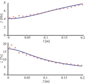
Fig. 7 The result of the modal test at zero towing speed.
The lateral tyre stiffnessk, tyre dampingd, the relaxation lengthσand the tor- sional dampingdtwere identified by measuring the natural frequency and damping ratio of the caster-wheel system for different caster lengths at zero towing speed.
In Fig.8, the results of the modal test are shown by red crosses while blue lines correspond to the fitted theoretical formulae. These can be expressed as
f= 1 2π
√ k(2
3a3+ 2(aσ+l2)(a+σ)) JA
, (27)
and
ζ = π
f ·dt+d(2
3a3+ 2(aσ+l2)(a+σ)) JA
. (28)
The parameters of the implemented Coulomb friction law are defined here by the maximum of the transmittable lateral force for sticking and sliding respectively:
Frmax = µrFz and Fsmax = µsFz. These were set to match the measured and simulated non-linear vibration amplitudes. The identified system parameters of the experiments are listed in Table 2.
5.2 Steady state behaviour
The steady-state behaviour of the non-smooth delayed tyre model was also tested and compared to experiments. For this purpose the lateral tyre force was measured while the deflection angleψ(equal to the side-slip angle in steady-state) was held
constant. Thus, the steady state force characteristics was generated as shown in Fig. 8. Using the measurement data the parameters BF, CF, DF and EF are identified in the Magic Formula [1]:
F(α) =−DFsin (CFarctan (BFα−EF(BFα−arctan (BFα)))). (29) With the help of steady-state measurements the coefficients in the Magic Formula were identified as BF = 3.9085, CF = 1.55, DF = 119.12 N, EF = 0.3924. In Fig. 8, the Magic Formula is compared to numerical simulations using the non- smooth delayed tyre model shown by thick black curves while the simulated self aligning moment characteristics is also shown (although this was not measured).
It can be seen that the transition from partial sliding to full sliding is less smooth than the measurement data show. This can be explained by the relative stiffness of the stretched string model for sliding. This is presumably also the main reason why the simulated forces corresponding to the same deflection angles are higher than the measured ones, although in our measurement set-up the vertical load also decreases in some extent for large tyre deformation which also results a smaller maximum of the lateral force. In Fig. 8 the lateral forces are normalised by their maximum values, so this effect cannot be observed there. Another difference is that while the characteristics obtained using the stretched string model saturates at its maximum value, the measured force shows a minimal backdrop for large side slip angles which is usually explained by the difference between the friction coefficients for rolling and sliding. Using the stretched string model this effect practically never shows up in the non-smooth delayed tyre model as the sliding regions spread rapidly from the end of the contact patch and no such rolling region is encountered where the lateral load is higher than the sliding limit.
To calculate the linear stability boundaries and the periodic solutions with the steady state tyre model we used the equation of motion given in Eqn. (1) with the ODE (10) for the leading point deformation. Thus, the dynamics of the tyre- ground contact was still considered in limited way while the lateral forceF was calculated from the Magic Formula (29). For the self-aligning moment a linear characteristics was used as
M =−κaBFCFDFα, (30)
where the parameterκis defined as κ=t∗awhere t∗=−CMα/CFα is the pneu- matic trail, that is the ratio of the torsional and lateral stiffness of the tyre for small deformation. In the meantime the side-slip angleα is calculated as
α=−arctanq(a, t)
σ . (31)
It is worth to mention that this assumption provides the quasi steady state straight- tangent approximation of the stretched string model [1].
5.3 Identification of the bistable regions
To capture the bistable parameter regions experimentally beginning from a domain where the straight-line motion is stable the speed of the conveyor belt was increased by steps of (approximately) 0.5 km/h until the stability boundary was crossed and
Fig. 8 Normalised tyre lateral force and self aligning torque characteristics. The light red stars represent the measurement data, the thick black curves correspond to the non-smooth delayed tyre model, while the thin grey curve corresponds to the Magic Formula.
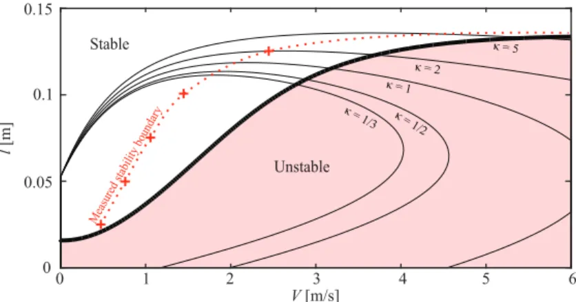
0 1 2 3 4 5 6
V [m/s]
0 0.05 0.1 0.15
l [m]
Unstable Stable
κ = 1/
3 κ = 1/2 κ = 1
κ = 2
κ = 5
Meas ured
stability bo undary
Fig. 9 Measured and theoretical stability boundaries predicted by the stretched string model (thick black curve) and the Magic Formula (thin black curves). The shading refers to the stable/unstable behaviour of the stretched string model.
the system converged to a large amplitude limit-cycle. Then, to discover the limits of the bistable velocity-range, the conveyor belt speed was decreased until the vibrations disappeared.
First, the measurement results were compared to the linear stability boundaries obtained from the non-smooth delay and the Magic Formula tyre model as shown in Fig. 9. Since the self aligning torque was not measured we present the stability boundaries for various pneumatic trails varying the parameterκfrom 1/3 to 5. It can be seen that the stretched string model and the quasi steady state tyre model have both have an error in the critical velocity compared to the measurements
Stable
Unstable Stretched string
simulated amplitudes
Measured amplitudes 0
0.5 1 1.5
2 2.5
0 0.5 1 1.5 2 2.5
ψ [rad]
0 0.05
0.1 l [m]
V [m/s]
Bistable (measured)
Bistable (simulated, stretched string)
0 0.5 1 1.5 2 2.5
Magic formula, κ = 5
Magic formula stability boudary, no bistable domain
{
{
Magic formula, κ = 1 Magic formula, κ = 1/3
κ = 5 κ = 1 κ = 1/3
κ = 1/3
Fig. 10 Measured and theoretical vibration amplitudes (upper panel) and theoretical linear stability chart of the rectilinear motion (lower panel). In the upper panel blue crosses cor- respond to the amplitudes simulated with the stretched string tyre model, the red ones to measured results, while the thin black curves show the amplitudes obtained with the Magic Formula. In the lower stability chart in the plane of the towing velocity V and the caster lenghtlthe thick black curve shows the stability boundary with the stretched string model.
The white (unstable) and the red (stable) domain refers to the results with the NSDTM. Sta- bility boundaries predicted by the steady-state tyre model are shown by thin black curves.
The thick orange segments of thel= 0.075 m line shows the measured and simulated bistable parameter regions.
Parameter Notation Value
Mass moment of inertia with respect to the joint A JA 0.179628 kgm2
Tyre-ground contact patch half-length a 0.054 m
Tyre relaxation length σ 0.12 m
Distributed tyre stiffness k 43766 N/m2
Distributed tyre damping d 23 Ns/m2
Torsional damping at J dt 1.3 Nms
Maximum lateral force for rolling Frmax 900 N
Maximum lateral force for sliding Fsmax 600 N
Table 2 List of parameters of the experiments.
with the stretched string model providing an upper, whereas the Magic Formula a lower estimation for the stability boundary. It is also visible though that for smaller pneumatic trails the Magic Formula provides an upper critical speed above which it predicts the rectilinear motion to be stable. Such behaviour was not experienced during the measurements in the velocity range of V = 0−5 m/s.
The stability boundaries are more in accordance with the experimental results for higher pneumatic trails. Nevertheless, a pneumatic trail around five times the contact patch half length is physically unimaginable as the lever of the resultant force would exceed even the contact patch and the relaxation length together.
Although this discrepancy could be overcome by choosing an even higher relaxation length as well. This, however, would result the unstable domain spreading to higher caster lengths as well where in the experiments the rectilinear motion was found to be stable.
The results of the measurements are compared with numerical simulations as well, where the same process was simulated using the non-smooth delayed tyre model to cover the bistable parameter range. The measured and simulated vibra- tion amplitudes are shown for the caster length of l = 0.075 m in Fig. 10. The arrows above the measured and simulated data indicate the hysteresis loop re- garding the stability of the rectilinear motion. As it can be observed, during the experiment the rectilinear motion lost its stability at a lower velocity than is can be predicted by numerical simulation. Comparing the width of the measured and simulated bistable zones one can see that the measurement provided a narrower unsafe domain. Amongst many other effects this can be explained by the fact that the measurements were affected by the noise from the conveyor belt and the wheel unbalance which, by providing large enough perturbation, could un-stabilise the straight-line motion. Otherwise the shift of the stability boundary towards a lower velocity level can be also explained by the yet unexplored velocity-dependence of the tyre properties. Such a proprety is suggested by the much stronger velocity- dependence of the vibration amplitudes than the simulation results show. Moreover the behaviour of the rubber tyre is influenced by many non-modelled factors, such as the already mentioned velocity dependence as well as material non-linearities and the tyre and conveyor belt temperature. We also present the amplitudes of the periodic solutions with the Magic Formula tyre model for different pneumatic trails which were calculated by using the continuation software AUTO07p [18].
In this case larger discrepancies were found in the vibration amplitudes for larger pneumatic trails, while we found better match forκ= 1/3, which can be explained by the fact that for large deformations the pneumatic trail becomes indeed smaller.
It can be also seen though, that the Magic Formula tyre model in our mechanical model does not result a bistable parameter domain.
6 CONCLUSIONS
In the paper we presented a non-smooth delayed tyre model to describe the lateral deformation of the tyre in the tyre-road contact region. The model was imple- mented in the in-plane mechanical model of a towed wheel and was used to study the nonlinear dynamics of wheel-shimmy. With the help of numerical simulations we demonstrated how the memory effect and the partial side-slip in the contact patch cause a hysteresis effect regarding the stability of the straight-line motion.
It is worth to mention that while the nonlinear dynamics of wheel-shimmy has been analysed in many studies using quasi steady-state tyre model [16], or a sim- plified version of the stretched-string model like Von Schlippe’s approximation in [17], a subcritical Hopf bifurcation seems to occur only if both the delay and the friction are taken into account in the contact. This is also verified by our anal- ysis demonstrating that although the lateral force generated in steady-state by the semi empirical Magic Formula tyre model was in better accordance with the measurements it does not provide a bistable parameter domain beside the linearly unstable region as experienced in measurements.
With the non-smooth delayed tyre model the simplifications of considering slid- ing regions at the leading and rear edges only enabled us to compose a multi-scale method which provides results with good accuracy within a manageable compu- tation time. Therefore, the presented code may be worth to be optimised further with respect to the computation time to achieve close to real-time computing.
Moreover, based on this idea, a similar method could be developed to calculate the sliding zones for the longitudinal deformations of the tyre, which would enable us to create more accurate algorithms which are capable of working together with anti-lock braking systems.
The presented numerical simulation is capable to find the stable solutions in the system (equilibria and periodic orbits). Thus, it enabled us to capture the hys- teresis effect in the stability of the rectilinear motion which was also confirmed by experiments with good qualitative agreement with the simulations. Nevertheless, the measurements on the conveyor belt also revealed inaccuracies in our model which could be addressed after further investigation of the presumably significant effect of the velocity and the temperature on the tyre behaviour.
Although our current algorithm has some limitations identifying the unstable solutions of the system, it may be used as a basis for the continuation of the limit cycles. Shooting or control-based continuation algorithms in further research would be capable to reveal the structure of the global bifurcation in the system in more detail.
References
1. Pacejka, H.B., Tyre and Vehicle Dynamics, Elsevier Butterworth-Heinemann, 2002.
2. Rill, G., TMeasyThe handling tire model for all driving situations, in Proceed- ings of the XV International Symposium on Dynamic Problems of Mechanics, Buzios, RJ, Brazil, 2013.
3. Tak´acs, D., Orosz, G., St´ep´an, G., Delay effect in shimmy dynamics of wheels with stretched string-like tyres, European Journal of Mechanics A/Solids, 28, 516-525, 2009.
4. Tak´acs, D., St´ep´an, G., Contact patch memory of tyres leading to lateral vibrations of four-wheeled vehicles, Philosophical Transactions of the Royal Society A: Mathematical, Physical and Engineering Sciences, 371, 2013.
5. Lugner, P., Pacejka, H. B., Pl¨ochl, M., Recent advances in tyre models and testing procedures, Vehicle System Dynamics, Vol. 43, pp. 413-426, 2005.
6. Besselink, I.J.M,, Schmeitz, A.J.C., Pacejka, H.B., An improved Macig For- mula/Swift tyre model that can handle inflation pressure changes, Vehicle System Dynamics, 48, 332-352, 2010.
7. Gipser, M., FTire – the tire simulation model for all applications related to vehicle dynamics, Vehicle System Dynamics, Vol. 45, pp. 139-151, 2007.
8. Oertel, Ch., On modelling contact and friction - calculation of tyre response on uneven roads. Proceedings and 2nd Colloquium on Tyre Models for Vehicle Analysis, International Journal of Vehicle System Dynamics, Vol 27 (Suppl.), 1996.
9. H¨olscher, H., Tewes, M., Botkin, N., L¨ohndorf, M., Hoffmann, K., Quandt, E-, Modeling of pneumatic tires by a finite element model for the development a tire friction remote sensor, Computers and Structures, 2004.
10. Korunovic, N., Trajanovic, M., Stojkovic, M., Misic, D., Milovanovic, J., Finite element analysis of a tire steady rolling on the drum and comparison with experiment, Journal of Mechanical Engineering, 2011.
11. Tak´acs, D., St´ep´an, G., Micro-shimmy of towed structures in experimentally uncharted unstable parameter domain, Vehicle System Dynamics, Vol. 50, pp.
1613-1630, 2012.
12. Thaitirarot, A., Flicek, R., Hills, D.A., Barber, J.R., The use of static reduc- tion in the solution of two-dimensional frictional contact problems, Journal of Mechanical Engineering Science, Vol. 228, pp. 1474–1487., 2014.
13. Segel, L., Force and moment response of pneumatic tires to lateral motion inputs Journal of Engineering for Industry, Transactions of the ASME, Vol.
88B, pp. 37-44, 1966.
14. Kuznetsov, Y., Elements of Applied Bifurcation Theory, Springer-Verlag New York, 2004.
15. Leine, R.I., Bifurcations of equilibria in non-smooth continuous system, Phys- ica D, 223, 121-137, 2006.
16. Ran, S., Besselink, I. J. M., Nijmeijer, H., Applications of nonlinear tyre mmodel to analyse shimmy Vehicle System Dynamics, Vol. 52, pp. 387-404, 2014.
17. Howcroft, C., Lowenberg, M., Neild, S., Krauskopf, B., Coetzee, E., Shimmy of an Aircraft Main Landing Gear With Geometric Coupling and Mechanical Freeplay, Journal of Computational and Nonlinear Dynamics, Vol. 10, 2015.
18. Doedel, E. J., Oldeman, B. E., AUTO-07p: Continuation and bifurcation soft- ware for ordinary differential equations, Concordia University, Montreal, 2012.