Enumeration of Fuss-skew paths

Enumeration of Fuss-skew paths

Toufik Mansour

, José Luis Ramírez

aDepartment of Mathematics, University of Haifa, 3498838 Haifa, Israel

tmansour@univ.haifa.ac.il

bDepartamento de Matemáticas,

Universidad Nacional de Colombia, Bogotá, Colombia jlramirezr@unal.edu.co

Submitted: December 22, 2021 Accepted: January 14, 2022 Published online: January 29, 2022

Abstract

In this paper, we introduce the concept of a Fuss-skew path and then we study the distribution of the semi-perimeter, area, peaks, and corners statistics. We use generating functions to obtain our main results.

Keywords:Skew Dyck path, Fuss-Catalan numbers, generating function AMS Subject Classification:05A15, 05A19

1. Introduction

A skew Dyck path is a lattice path in the first quadrant that starts at the origin, ends on the 𝑥-axis, and consists of up-steps 𝑈 = (1,1), down-steps 𝐷 = (1,−1), and left-steps 𝐿 = (−1,−1), such that up and left steps do not overlap. The definition of skew Dyck path was introduced by Deutsch, Munarini, and Rinaldi [4]. Some additional results about skew Dyck path can be found in [2, 5, 8, 14].

Let 𝑠𝑛 denote the number of skew Dyck path of semilength 𝑛, where the semilength of a path is defined as the number its up-steps. The sequence 𝑠𝑛 is given by the combinatorial sum 𝑠𝑛 =∑︀𝑛

𝑘=1

(︀_𝑛−1

𝑘−1

)︀𝑐𝑘, where 𝑐𝑛 = _𝑛+1¹ (︀2𝑛 𝑛

)︀ is the 𝑛-th Catalan number. The sequence𝑠𝑛 appears in OEIS as A002212 [15], and its first few values are

1, 1, 3, 10, 36, 137, 543, 2219, 9285, 39587.

doi: https://doi.org/10.33039/ami.2022.01.001 url: https://ami.uni-eszterhazy.hu

1

One way to generalize the classical Dyck paths is to regard the length of an up-step 𝑈 as a parameter. Given a positive number ℓ, an ℓ-Dyck path is a lattice path in the first quadrant from (0,0) to ((ℓ+ 1)𝑛,0) where 𝑛≥0 using up-steps 𝑈ℓ = (ℓ, ℓ) and down-steps 𝑈 = (1,−1). For ℓ = 1, we recover the classical Dyck path. The total number of ℓ-Dyck path with length (ℓ+ 1)𝑛 is given by 𝑐ℓ(𝑛) = _𝑡𝑛+1¹ (︀_(𝑡+1)𝑛

𝑛

)︀(cf. [1]). We will refer toℓ-Dyck paths here as the “Fuss” case because the sequence𝑐ℓ(𝑛)was first investigated by N. I. Fuss (see, for example, [7, 16] for several combinatorial interpretations for both the Catalan and Fuss-Catalan numbers).

Our focus in this paper is to introduce a Fuss analogue of the skew Dyck path.

Given a positive integerℓ, anℓ-Fuss-skew path is a path in the first quadrant that starts at the origin, ends on the𝑥-axis, and consists of up-steps𝑈ℓ= (ℓ, ℓ), down- steps𝐷= (1,−1), and left steps𝐿= (−1,−1), such that up and left steps do not overlap. Given anℓ-Fuss-skew path𝑃, we define the semilength of𝑃, denote by

|𝑃|, as the number of up-steps of 𝑃. For example, Figure 1 shows a 3-Fuss-skew path of semilength6. It is clear that the1-Fuss-skew paths coincide with the skew Dyck paths. Let S^𝑛,ℓ denote the set of allℓ-Fuss-skew path of semilength 𝑛, and S^ℓ=⋃︀

𝑛≥0S^𝑛,ℓ. For example, Figure 4 shows all the paths inS^2,2.

(20,0) (0,0)

Figure 1. 3-Fuss-skew path of semilength 6.

2. Counting special steps

For a given path 𝑃 ∈ Sℓ, we use 𝑢(𝑃), 𝑑(𝑃), and 𝑡(𝑃) to denote the number of up-steps, down-steps, and left-steps of 𝑃, respectively. In this section, we study the distribution of these parameters overSℓ. Using these parameters, we define the generating function

𝐹ℓ(𝑥, 𝑝, 𝑞) := ∑︁

𝑃∈S^ℓ

𝑥^𝑢(𝑃)𝑝^𝑑(𝑃)𝑞^𝑡(𝑃).

For simplicity, we use𝐹ℓto denote the generating function𝐹ℓ(𝑥, 𝑝, 𝑞).

Theorem 2.1. The generating function𝐹ℓ(𝑥, 𝑝, 𝑞)satisfies the functional equation 𝐹ℓ= 1 +𝑥(𝑝𝐹ℓ+𝑞)^ℓ−1(𝑝𝐹_ℓ²+𝑞(𝐹ℓ−1)). (2.1)

Proof. Let𝒜^𝑖 denote theℓ-Fuss-skew paths whose last𝑦-coordinate is𝑖and let𝐴𝑖

denote the generating function defined by 𝐴𝑖= ∑︁

𝑃∈𝒜𝑖

𝑥^𝑢(𝑃)𝑝^𝑑(𝑃)𝑞^𝑡(𝑃).

A non-empty ℓ-Fuss-skew path can be uniquely decomposed as either𝑈ℓ𝑇 𝐷𝑃 or 𝑈ℓ𝑇 𝐿, where𝑈ℓ𝑇 is a lattice path in𝒜¹and𝑃 is anℓ-Fuss-skew path (see Figure 2 for a graphical representation of this decomposition). From this decomposition, we obtain the functional equation (cf. [6])

𝐹ℓ= 1 +𝑥(𝑝𝐴1𝐹ℓ+𝑞𝐴1). (2.2)

ℓ

1

ℓ

1

Figure 2. Decomposition of aℓ-Fuss-skew path.

The paths of 𝒜^𝑖 can be decomposed as 𝑇 𝐷𝑃 or 𝑇 𝐿, where 𝑇 ∈ 𝒜^𝑖+1 for 𝑖 = 1, . . . , ℓ−2 and 𝑃 ∈ S^ℓ (see Figure 3 for a graphical representation of this decomposition). Moreover, the paths of 𝒜ℓ−1 are decomposed as 𝑃1𝐷𝑃2 or 𝑃^′𝐿, where𝑃1, 𝑃2, 𝑃^′∈S^ℓ and𝑃^′ is non-empty.

ℓ _{i+ 1} ℓ _{i+ 1}

i i

Figure 3. Decomposition of the paths in𝒜^𝑖.

From the above decompositions, we obtain the functional equations

𝐴𝑖=𝑝𝐴𝑖+1𝐹ℓ+𝑞𝐴𝑖+1, for 𝑖= 1, . . . , ℓ−2, and 𝐴ℓ−1=𝑝𝐹_ℓ²+𝑞(𝐹ℓ−1).

Note that in these functional equations we do not consider the first up-step because it was considered in (2.2). Therefore, we have

𝐹ℓ= 1 +𝑥(𝑝𝐹ℓ+𝑞)𝐴1= 1 +𝑥(𝑝𝐹ℓ+𝑞)²𝐴2

=· · ·= 1 +𝑥(𝑝𝐹ℓ+𝑞)^ℓ−1(𝑝𝐹_ℓ²+𝑞(𝐹ℓ−1)).

Let 𝑠ℓ(𝑛, 𝑝, 𝑞) denote the joint distribution over S^𝑛,ℓ for the number of down and left steps, that is,

𝑠ℓ(𝑛, 𝑝, 𝑞) = ∑︁

𝑃∈S𝑛,ℓ

𝑝^𝑑(𝑃)𝑞^𝑡(𝑃).

It is clear that𝐹ℓ=∑︀

𝑛≥0𝑠ℓ(𝑛, 𝑝, 𝑞)𝑥^𝑛. From the Lagrange inversion theorem (see for instance [13]), we give a combinatorial expression for the sequence𝑠ℓ(𝑛, 𝑝, 𝑞).

Theorem 2.2. For𝑛≥1, the sequence𝑠ℓ(𝑛, 𝑝, 𝑞)is given by

1 𝑛

∑︁𝑛

𝑗=0

∑︁𝑗

𝑘=0

(︂𝑛 𝑗

)︂(︂𝑗 𝑘

)︂(︂ 𝑛(ℓ−1) 𝑛−2𝑗+𝑘−1

)︂

𝑝^{2𝑛−1−2𝑗}(2𝑝+𝑞)^𝑘(𝑝+𝑞)^{𝑛(ℓ−2)+2𝑗−𝑘+1}.

In particular, the total number of ℓ-Fuss-skew paths of semilength 𝑛is

𝑠ℓ(𝑛) :=𝑠ℓ(𝑛,1,1) = 1 𝑛

∑︁𝑛

𝑗=0

∑︁𝑗

𝑘=0

(︂𝑛 𝑗

)︂(︂𝑗 𝑘

)︂(︂ 𝑛(ℓ−1) 𝑛−2𝑗+𝑘−1

)︂

3^𝑘2^{𝑛(ℓ−2)+2𝑗−𝑘+1}.

Proof. The functional equation given in Theorem 2.1 can be written as 𝑄ℓ=𝑥(𝑝(𝑄ℓ+ 1) +𝑞)^ℓ−1(𝑝(𝑄ℓ+ 1)²+𝑞𝑄ℓ),

where𝑄ℓ=𝐹ℓ−1. From the Lagrange inversion theorem, we deduce

[𝑥^𝑛]𝐻ℓ= 1

𝑛[𝑧^𝑛−1](𝑝(𝑧+ 1) +𝑞)^{(ℓ−1)𝑛}(𝑝(𝑧+ 1)²+𝑞𝑧)^𝑛

= 1

𝑛[𝑧^𝑛−1]∑︁

𝑠≥0

(︂(ℓ−1)𝑛 𝑠

)︂

(𝑝𝑧)^𝑠(𝑝+𝑞)^{(ℓ−1)𝑛−𝑠}(𝑝𝑧²+ (2𝑝+ 1)𝑧+𝑝)^𝑛

= 1

𝑛[𝑧^𝑛−1]∑︁

𝑠≥0

(︂(ℓ−1)𝑛 𝑠

)︂

(𝑝𝑧)^𝑠(𝑝+𝑞)^{(ℓ−1)𝑛−𝑠}

×

∑︁𝑛

𝑗=0

∑︁𝑗

𝑘=0

(︂𝑛 𝑗

)︂(︂𝑗 𝑘

)︂

𝑝^𝑛−𝑗((2𝑝+𝑞)𝑧)^𝑘(𝑝𝑧²)^𝑗−𝑘

= 1 𝑛

∑︁𝑛

𝑗=0

∑︁𝑗

𝑘=0

(︂𝑛 𝑗

)︂(︂𝑗 𝑘

)︂(︂ 𝑛(ℓ−1) 𝑛−2𝑗+𝑘−1

)︂

𝑝^{2𝑛−1−2𝑗}(2𝑝+𝑞)^𝑘(𝑝+𝑞)^{𝑛(ℓ−2)+2𝑗−𝑘+1}.

For example, Figure 4 shows all 2-Fuss-skew paths of semilength 2 counted by the term𝑠ℓ(2, 𝑝, 𝑞) = 3𝑝⁴+ 6𝑝³𝑞+ 4𝑝²𝑞²+𝑝𝑞³.

p⁴

p³q

p³q

p²q²

p³q p²q² p²q²

pq³

p⁴

p³q p³q p²q²

p⁴

p³q

Figure 4. 2-Fuss-skew paths counted by𝑠ℓ(2, 𝑝, 𝑞).

From Theorem 2.2, we obtain that the total number of down-steps over the ℓ-Fuss-skew paths of semilength 𝑛is given by

𝜕𝑠ℓ(𝑛, 𝑝,1)

𝜕𝑝

⃒⃒

⃒⃒_𝑝=1

= 1 𝑛

∑︁𝑛

𝑗=0

∑︁𝑗

𝑘=0

(︂𝑛 𝑗

)︂(︂𝑗 𝑘

)︂(︂ 𝑛(ℓ−1) 𝑛−2𝑗+𝑘−1

)︂

2(ℓ−2)𝑛+2𝑗−𝑘3^𝑘−1(3𝑛(ℓ+ 2) +𝑘−6𝑗−3).

Moreover, the total number of left-steps over theℓ-Fuss-skew paths of semilength 𝑛is

𝜕𝑠ℓ(𝑛,1, 𝑞)

𝜕𝑞

⃒⃒

⃒⃒

𝑞=1

= 1 𝑛

∑︁𝑛

𝑗=0

∑︁𝑗

𝑘=0

(︂𝑛 𝑗

)︂(︂𝑗 𝑘

)︂(︂ 𝑛(ℓ−1) 𝑛−2𝑗+𝑘−1

)︂

2(ℓ−2)𝑛+2𝑗−𝑘3^𝑘−1(3𝑛(ℓ−2)−𝑘+ 6𝑗+ 3).

Equation (2.1) can be explicitly solved for ℓ = 1. In this case, we obtain the generating function

𝐹1(𝑥, 𝑝, 𝑞) = 1−𝑞𝑥−√︀

(1−𝑞𝑥)(1−(4𝑝+𝑞)𝑥)

2𝑝𝑥 .

Moreover, the generating functions for the total number of down-steps (A026388) and left steps (A026376) over the skew-Dyck paths are respectively

1−4𝑥+ 3𝑥²−√

1−6𝑥+ 5𝑥²(1−𝑥) 2𝑥√

1−6𝑥+ 5𝑥²

and

1−3𝑥−√

1−6𝑥+ 5𝑥² 2√

1−6𝑥+ 5𝑥² . Notice that we recover some of the results of [5].

Finally, Table 1 shows the first few values of the total number ofℓ-Fuss-skew paths of semilength𝑛.

Table 1. Values of𝑠ℓ(𝑛,1,1)for1≤ℓ≤5,𝑛= 1, . . . ,7.

ℓ∖𝑛 1 2 3 4 5 6 7

ℓ= 1 1 3 10 36 137 543 2219

ℓ= 2 2 14 118 1114 11306 120534 1331374

ℓ= 3 4 64 1296 29888 745856 19614464 535394560 ℓ= 4 8 288 13568 734720 43202560 2681634816 172936069120

2.1. The width of a path

For a given path 𝑃 ∈ S^ℓ, we define the width of 𝑃, denoted by 𝜈(𝑃), as the 𝑥- coordinate of the last point of 𝑃. For example, the width of the path given in Figure 1 is 20. We define the generating function

𝐺ℓ(𝑥, 𝑦) :=𝐺ℓ= ∑︁

𝑃∈S^ℓ

𝑥^𝑢(𝑃)𝑦^𝜈(𝑃).

Note that each𝑈ℓ and𝐷 step of a path increases the width byℓunits and 1 unit, respectively, while the left-step 𝐿 decreases the width by 1 unit. Therefore, we have the functional equation

𝐺ℓ= 1 +𝑥𝑦^ℓ(𝑦𝐺ℓ+𝑦⁻¹)^ℓ−1(𝑦𝐺²_ℓ+𝑦⁻¹(𝐺ℓ−1))

= 1 +𝑥(𝑦²𝐺ℓ+ 1)^ℓ−1(𝑦²𝐺²_ℓ+ (𝐺ℓ−1)). (2.3) Let𝑔ℓ(𝑛, 𝑦)denote the distribution overS^𝑛,ℓ for the width parameter, i.e.,

𝑔ℓ(𝑛, 𝑦) = ∑︁

𝑃∈S^𝑛,ℓ

𝑦^𝜈(𝑃).

From the functional equation (2.3) and the Lagrange inversion theorem, we obtain the following theorem.

Theorem 2.3. For𝑛≥1, the sequence𝑔ℓ(𝑛, 𝑦)is given by

1 𝑛

∑︁𝑛

𝑗=0

∑︁𝑗

𝑘=0

(︂𝑛 𝑗

)︂(︂𝑗 𝑘

)︂(︂ 𝑛(ℓ−1) 𝑛−2𝑗+𝑘−1

)︂

𝑦^{4(𝑛−𝑗)−2}(𝑦²+ 1)^{𝑛(ℓ−2)+2𝑗−𝑘+1}(2𝑦²+ 1)^𝑘.

For example, 𝑔2(2, 𝑦) =𝑦²+ 4𝑦⁴+ 6𝑦⁶+ 3𝑦⁸. This polynomial can be found from the paths in Figure 4. For ℓ= 1, we obtain the explicit generating function with respect to the width of a skew Dyck path.

𝐺1(𝑥, 𝑦) = 1−𝑥−√︀

(1−𝑥)(1−𝑥−4𝑥𝑦²)

2𝑥𝑦² .

3. Number of peaks

For a given path𝑃 ∈S^ℓ, we define thepeaksof𝑃, denoted by𝜌(𝑃), as the number of subpaths of the form𝑈ℓ𝐷 (for counting peaks in a Dyck path, for example, see [9, 11]). For example, the number of peaks of the path given in Figure 1 is 5. We define the generating function

𝑃ℓ(𝑥, 𝑦) :=𝑃ℓ= ∑︁

𝑃∈Sℓ

𝑥^𝑢(𝑃)𝑦^𝜌(𝑃).

Theorem 3.1. The generating function𝑃ℓ(𝑥, 𝑦)satisfies the functional equation 𝑃ℓ= 1 +𝑥(𝑃ℓ+ 1)^ℓ−1((𝑃ℓ−1 +𝑦)𝑃ℓ+ (𝑃ℓ−1)).

Proof. Let𝐶𝑖 denote the generating function defined by 𝐶𝑖 =∑︀

𝑃∈𝒜𝑖𝑥^𝑢(𝑃)𝑦^𝜌(𝑃). From the decomposition given for the ℓ-Fuss-skew paths, we have the equation 𝑃ℓ= 1 +𝑥(𝐶1𝑃ℓ+𝐶1). Moreover,

𝐶𝑖=𝐶𝑖+1𝑃ℓ+𝐶𝑖+1, for𝑖= 1, . . . , ℓ−2, and 𝐶ℓ−1= (𝑃ℓ−1 +𝑦)𝑃ℓ+ (𝑃ℓ−1).

From these relations, we obtain the desired result.

Let𝑝ℓ(𝑛, 𝑦)denote the distribution overS^𝑛 for the peaks statistic, i.e., 𝑝ℓ(𝑛, 𝑦) = ∑︁

𝑃∈S^𝑛

𝑦^𝜌(𝑃).

From the Lagrange inversion theorem, we deduce the following result.

Theorem 3.2. For𝑛≥1, we have

𝑝ℓ(𝑛, 𝑦) = 1 𝑛

∑︁𝑛

𝑗=0

∑︁𝑗

𝑘=0

(︂𝑛 𝑗

)︂(︂𝑗 𝑘

)︂(︂ 𝑛(ℓ−1) 𝑛−2𝑗+𝑘−1

)︂

2^{𝑛(ℓ−2)+2𝑗−𝑘+1}𝑦^𝑛−𝑗(𝑦+ 2)^𝑘.

In particular, the total number of peaks in allℓ-Fuss-skew paths of semilength 𝑛is

𝜕𝑝ℓ(𝑛, 𝑦)

𝜕𝑦

⃒⃒

⃒⃒

𝑦=1

= 1 𝑛

∑︁𝑛

𝑗=0

∑︁𝑗

𝑘=0

(︂𝑛 𝑗

)︂(︂𝑗 𝑘

)︂(︂ 𝑛(ℓ−1) 𝑛−2𝑗+𝑘−1

)︂

2^{𝑛(ℓ−2)+2𝑗−𝑘+1}3^𝑘−1(3(𝑛−𝑗) +𝑘).

For example,𝑝2(2, 𝑦) = 8𝑦+ 6𝑦². This polynomial can be found from the paths in Figure 4. Forℓ= 1 we obtain the generating function

𝑃1(𝑥, 𝑦) = 1−𝑥𝑦−√︀

(1−𝑥𝑦)²−4(1−𝑥)𝑥

2𝑥 .

Moreover, the generating function for the total number of peaks is 1−𝑥−√

1−6𝑥+ 5𝑥² 2√

1−6𝑥+ 5𝑥² .

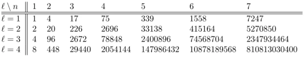
Table 2 shows the first few values of the number of peaks inℓ-Fuss-skew paths of semilength𝑛.

Table 2. Total number of peaks inS^ℓ.

ℓ∖𝑛 1 2 3 4 5 6 7

ℓ= 1 1 4 17 75 339 1558 7247

ℓ= 2 2 20 226 2696 33138 415164 5270850

ℓ= 3 4 96 2672 78848 2400896 74568704 2347934464 ℓ= 4 8 448 29440 2054144 147986432 10878189568 810813030400

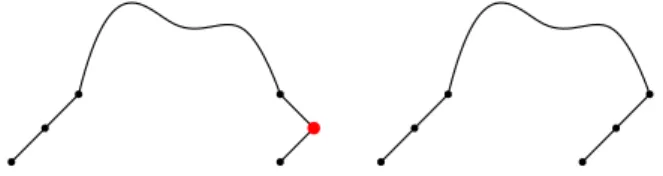
4. Number of corners

For a given path 𝑃 ∈S^ℓ, we define acorner of 𝑃 as a right angle caused by two consecutive steps in the graph of 𝑃. For example, the path given in Figure 5 has 4 corners, depicted in red. This statistic has been studied in other combinatorial structures as integer partitions [3], compositions [10], and bargraphs [12].

Figure 5. Corners of a path.

Let𝜏(𝑃)denote the number of corners of𝑃. We define the bivariate generating function

𝑊ℓ(𝑥, 𝑦) :=𝑊ℓ= ∑︁

𝑃∈Sℓ

𝑥^𝑢(𝑃)𝑦^𝜏(𝑃).

In this section, we analyze the casesℓ= 1andℓ= 2. We leave as an open question the case ℓ≥3.

Theorem 4.1. The generating function𝑊1(𝑥, 𝑦)satisfies the functional equation 𝑥𝑦(1 +𝑦)𝑊₁³−(2−𝑥(2−𝑦²))𝑊₁²+ 3(1−𝑥)𝑊1+𝑥−1 = 0.

Proof. Let𝒟andℒdenote the skew Dyck paths whose last step is a down-step or a left-step, respectively. Let 𝐷and𝐿 denote the generating functions defined by

𝐷= ∑︁

𝑃∈𝒟

𝑥^𝑢(𝑃)𝑦^𝜏(𝑃) and 𝐿=∑︁

𝑃∈ℒ

𝑥^𝑢(𝑃)𝑦^𝜏(𝑃).

A non-empty skew Dyck path can be uniquely decomposed as either 𝑈 𝑇1𝐿 or 𝑈 𝑇2𝐷𝑇3, where 𝑇1, 𝑇2, and 𝑇3 are lattice paths inS1 with𝑇1 non-empty. In the first case,𝑇1has two options: the last step is a down-step or a left step, see Figure 6.

Then, this case contributes to the generating function the term𝑥(𝑦𝐷+𝐿).

Figure 6. Decomposition of a skew Dyck path.

On the other hand,𝑇2can be an empty path or a path in𝒟orℒ. If𝑇3is empty, then this case contributes to the generating function the term𝑥(𝑦+𝐷+𝐿𝑦). On the other hand, if the path 𝑇3 is non-empty, then this case contributes to the generating function the term𝑥(𝑦+𝐷+𝑦𝐿)𝑦(𝑊1−1), see Figure 7. Summarizing these cases, we obtain the functional equation

𝑊1= 1 +𝑥(𝑦𝐷+𝐿) +𝑥(𝑦+𝐷+𝑦𝐿)(1 +𝑦(𝑊1−1)).

From a similar argument, we obtain the equations

𝐷=𝑥(𝑦+𝐷+𝑦𝐿)(1 +𝑦𝐷) and 𝐿=𝑥(𝑦𝐷+𝐿) +𝑥(𝑦+𝐷+𝑦𝐿)(𝑦𝐿).

Figure 7. Decomposition of a skew Dyck path.

Using the Gröbner basis on the polynomial equations for 𝑊1, 𝐷, and 𝐿, we obtain the desired result.

We can use a symbolic software computation to obtain the first few terms of the formal power series of𝑊1(𝑥, 𝑦)as follows:

𝑊1(𝑥, 𝑦) = 1 +𝑥𝑦+𝑥²(𝑦+𝑦²+𝑦³) +𝑥³(𝑦+ 2𝑦²+ 4𝑦³+ 2𝑦⁴+𝑦⁵) +𝑥⁴(𝑦+ 3𝑦²+ 9𝑦³+ 9𝑦⁴+ 10𝑦⁵+ 3𝑦⁶+𝑦⁷) +· · ·.

From the equation given in Theorem 4.1, we obtain

3𝑥𝑆³(𝑥) + 6𝑥𝑆²(𝑥)𝐾(𝑥)−2𝑥𝑆²(𝑥)−2(2−𝑥)𝑆(𝑥)𝐾(𝑥) + 3(1−𝑥)𝐾(𝑥) = 0, where 𝐾(𝑥) is the generating function for the total number of corners in skew Dyck paths and 𝑆(𝑥) = (1−𝑥−√

1−6𝑥+ 5𝑥²)/(2𝑥) is the generating function for the number of the skew Dyck paths. Solving the above equation, we obtain the generating function

𝐾(𝑥) = 2(1−𝑥)(3 +𝑥)𝑥

(1−𝑥)(3−2𝑥)(1−5𝑥) + (3−11𝑥+ 4𝑥²)√

1−6𝑥+ 5𝑥²

=𝑥+ 6𝑥²+ 30𝑥³+ 145𝑥⁴+ 695𝑥⁵+ 3327𝑥⁶+ 15945𝑥⁷+· · · .

Theorem 4.2. The generating function𝑊2(𝑥, 𝑦)satisfies the functional equation 𝑥²𝑦⁴(1 +𝑦)³𝑊₂⁶−𝑥𝑦²(1 +𝑦)²(1−𝑥(1 + 6𝑦+𝑦²−3𝑦³))𝑊₂⁵

+𝑥𝑦(−4−7𝑦+ 3𝑦³+𝑥(1 +𝑦)²(4 + 9𝑦−11𝑦²−6𝑦³+ 3𝑦⁴))𝑊₂⁴

+ (4−2𝑥(1 +𝑦)²(4−7𝑦+𝑦²)−𝑥²(1 +𝑦)²(−4 + 2𝑦+ 21𝑦²−8𝑦³−5𝑦⁴+𝑦⁵))𝑊2³

+ (−12−𝑥²(1 +𝑦)²(8 + 4𝑦−18𝑦²+ 4𝑦³+𝑦⁴)−2𝑥(−10−9𝑦+ 6𝑦²+ 6𝑦³+𝑦⁴))𝑊2²

+ (12 +𝑥²(1 +𝑦)²(5 + 4𝑦−7𝑦²+𝑦³) +𝑥(−17−16𝑦+ 2𝑦²+ 4𝑦³+ 3𝑦⁴))𝑊2

+ (−4 +𝑥²(1 +𝑦)²(−1−𝑦+𝑦²) +𝑥(5 + 4𝑦−𝑦⁴)) = 0.

Proof. Let𝒟²andℒ²denote the 2-Fuss-skew paths whose last step is a down-step or a left-step, respectively. Let𝐷2 and𝐿2denote the generating functions defined by

𝐷2= ∑︁

𝑃∈𝒟2

𝑥^𝑢(𝑃)𝑦^𝜏(𝑃) and 𝐿2= ∑︁

𝑃∈ℒ2

𝑥^𝑢(𝑃)𝑦^𝜏(𝑃).

From a similar argument as in the proof of Theorem 4.1, we obtain the system of polynomial equations

𝑊2= 1 +𝑥((𝑦+𝑦𝐷2+𝐿2)(1 +𝑦²𝐷2+𝑦𝐿2)(1 +𝑦(𝑊2−1)) + (𝐷2+𝑦𝐿2) + (𝐷2+𝑦𝐿2)𝑦(1 +𝑦(𝑊2−1)) + (𝑦+𝑦𝐷2+𝐿2)(𝑦+𝑦𝐷2+𝑦²𝐿2)), 𝐷2=𝑥((𝑦+𝑦𝐷2+𝐿2)(1 +𝑦²𝐷2+𝑦𝐿2)𝑦𝐷2+ (𝐷2+𝑦𝐿2) + (𝐷2+𝑦𝐿2)𝑦(𝑦𝐷2)

+ (𝑦+𝑦𝐷2+𝐿2)(𝑦+𝑦𝐷2+𝑦²𝐿2)),

𝐿2=𝑥((𝑦+𝑦𝐷2+𝐿2)(1 +𝑦²𝐷2+𝑦𝐿2)(1 +𝑦𝐿2) + (𝐷2+𝑦𝐿2)𝑦(1 +𝑦𝐿2)).

By using the Gröbner basis, we obtain the desired result.

Expanding withMathematica the functional equation for𝑊2, we find 𝑊2(𝑥, 𝑦) = 1 + (𝑦+𝑦²)𝑥+ (𝑦+ 3𝑦²+ 5𝑦³+ 4𝑦⁴+𝑦⁵)𝑥²

+ (𝑦+ 5𝑦²+ 16𝑦³+ 27𝑦⁴+ 33𝑦⁵+ 25𝑦⁶+ 9𝑦⁷+ 2𝑦⁸)𝑥³+· · · .

Moreover, the first few terms of the total number of corners in S² are

3𝑥+43𝑥²+561𝑥³+7209𝑥⁴+92703𝑥⁵+1197151𝑥⁶+15532917𝑥⁷+202428373𝑥⁸+· · ·. From Figure 4 one can verify that there are 43 corners over all paths inS2,2.

5. Other generalization

Let H^ℓ denote the skew Dyck paths where left steps are below the line 𝑦 =ℓ. In particular, H⁰ are the Dyck path andH∞ are the skew Dyck path. We define the generating function

𝐻ℓ(𝑥, 𝑝, 𝑞) := ∑︁

𝑃∈H^ℓ

𝑥^𝑢(𝑃)𝑝^𝑑(𝑃)𝑞^𝑡(𝑃).

For simplicity, we use𝐻ℓ to denote the generating function𝐻ℓ(𝑥, 𝑝, 𝑞).

Theorem 5.1. Forℓ≥1, we have

𝐻ℓ= 1 +𝑞𝑥(𝐻ℓ−1−1) +𝑝𝑥𝐻ℓ−1𝐻ℓ, (5.1) with the initial value𝐻0= ^1−√_2𝑝𝑥^{1−4𝑝𝑥}.

Proof. A non-empty skew Dyck path inH^ℓcan be decomposed as𝑈 𝑇1𝐿or𝑈 𝑇2𝐷𝑇3, where𝑇1, 𝑇2∈H^ℓ−1with𝑇1a non-empty path, and𝑇3∈H^ℓ. From this decompo- sition follows the functional equation.

Recall that the 𝑚th Chebyshev polynomial of the second kind satisfies the recurrence relation𝑈𝑚(𝑡) = 2𝑡𝑈_𝑚−1(𝑡)−𝑈_𝑚−2(𝑡)with𝑈0(𝑡) = 1 and 𝑈1(𝑡) = 2𝑡.

Thus by induction onℓand Theorem 5.1, we obtain the following result.

Theorem 5.2. Let 𝑡 = ^1+𝑞𝑥

2√

𝑥(𝑝+𝑞−𝑝𝑞𝑥) and 𝑟=√︀

𝑥(𝑝+𝑞−𝑝𝑞𝑥). The generating function𝐻ℓ is given by

(𝑞𝑥𝑈𝑛−1(𝑡)−𝑟𝑈𝑛−2(𝑡))𝐶(𝑝𝑥) + (1−𝑞𝑥)𝑈𝑛−1(𝑡) 𝑈_𝑛−1(𝑡)−𝑟𝑈_𝑛−2(𝑡)−𝑝𝑥𝑈_𝑛−1(𝑡)𝐶(𝑝𝑥) ,

where𝑈𝑚is the𝑚th Chebyshev polynomial of the second kind and𝐶(𝑥) = ^1−√_2𝑥^1−4𝑥 the generating function for the Catalan numbers _𝑛+1¹ (︀2𝑛

𝑛

)︀.

The generating functions for the total number of skew Dyck path in H^ℓ for ℓ= 1,2,3are

𝐻1(𝑥,1,1) = 3−2𝑥−√ 1−4𝑥 1 +√

1−4𝑥 ,

𝐻2(𝑥,1,1) = 1 + 2𝑥−2𝑥²−(1−2𝑥)√ 1−4𝑥 1−𝑥−2(1−𝑥)𝑥+ (1 +𝑥)√

1−4𝑥, 𝐻3(𝑥,1,1) = 1−3𝑥+ 7𝑥²−4𝑥³+ (1 +𝑥−3𝑥²)√

1−4𝑥 1−4𝑥+ 2𝑥³+ (1 + 2𝑥²)√

1−4𝑥 .

Acknowledgements. We thanks Mark Shattuck for his comments on the previ- ous version of the paper.

References

[1] J.-C. Aval:Multivariate Fuss-Catalan numbers, Discrete Math. 308 (2008), pp. 4660–4669, doi:https://doi.org/10.1016/j.disc.2007.08.100.

[2] J. L. Baril,J. L. Ramírez,L. M. Simbaqueba:Counting prefixes of skew Dyck paths, J.

Integer Seq. Article 21.8.2 (2021).

[3] A. Blecher,C. Brennan,A. Knopfmacher,T. Mansour:Counting corners in parti- tions, Ramanujan J. 39 (2016), pp. 201–224,

doi:https://doi.org/10.1007/s11139-014-9666-4.

[4] E. Deutsch,E. Munarini,S. Rinaldi:Skew Dyck paths, J. Statist. Plann. Inference 140 (2010), pp. 2191–2203,

doi:https://doi.org/10.1016/j.jspi.2010.01.015.

[5] E. Deutsch,E. Munarini,S. Rinaldi:Skew Dyck paths, area, and superdiagonal bar- graphs, J. Statist. Plann. Inference 140 (2010), pp. 1550–1526,

doi:https://doi.org/10.1016/j.jspi.2009.12.013.

[6] P. Flajolet,R. Sedgewick:Analytic Combinatorics, Cambridge University Press, 2009.

[7] S. Heubach,N. Y. Li,T. Mansour:Staircase tilings and𝑘-Catalan structures, Discrete Math. 308 (2008), pp. 5954–5964,

doi:https://doi.org/10.1016/j.disc.2007.11.012.

[8] Q. L. Lu:Skew Motzkin paths, Acta Math. Sin. (Engl. Ser.) 33 (2017), pp. 657–667, doi:https://doi.org/10.1007/s10114-016-5292-y.

[9] T. Mansour: Counting peaks at height 𝑘 in a Dyck path, J. Integer Seq. Article 02.1.1 (2002).

[10] T. Mansour,A. S. Shabani,M. Shattuck:Counting corners in compositions and set partitions presented as bargraphs, J. Difference Equ. Appl. 24 (2018), pp. 992–1015, doi:https://doi.org/10.1080/10236198.2018.1444760.

[11] T. Mansour, M. Shattuck: Counting Dyck paths according to the maximum distance between peaks and valleys, J. Integer Seq. Article 12.1.1 (2012).

[12] T. Mansour,G. Yildirim: Enumerations of bargraphs with respect to corner statistics, Appl. Anal. Discrete Math. 14 (2020), pp. 221–238,

doi:https://dx.doi.org/10.2298/AADM181101009M.

[13] D. Merlini,R. Sprugnoli,M. C. Verri:Lagrange inversion: when and how, Acta Appl Math. 94 (2006), pp. 233–249,

doi:https://doi.org/10.1007/s10440-006-9077-7.

[14] H. Prodinger:Partial skew Dyck paths - A kernel method approach, arXiv:2108.09785v1 (2021),

doi:https://arxiv.org/abs/2108.09785v2.

[15] N. J. A. Sloane, The On-Line Encyclopedia of Integer Sequences, doi:https://oeis.org/.

[16] R. Stanley:Catalan Numbers, Cambridge University Press, 2015.