How to predict choice using eye-movements data?

(1)

Food Research International 143 (2021) 110309

Available online 15 March 2021

(http://creativecommons.org/licenses/by-nc-nd/4.0/).

How to predict choice using eye-movements data?

Attila Gere

^a^,^*

, K ´ aroly H ´ eberger

^b

, S ´ andor Kov ´ acs

^c

aInstitute of Food Science and Technology, Hungarian University of Agriculture and Life Sciences, H-1118 Budapest, Vill´anyi út. 29-31, Hungary

bPlasma Chemistry Research Group, ELKH Research Centre for Natural Sciences, H-1117 Budapest, Magyar tud´osok krt. 2, Hungary

cDepartment of Economic and Financial Mathematics, University of Debrecen, B¨osz¨orm´enyi út 138, H-4032 Debrecen, Hungary

A R T I C L E I N F O Keywords:

Decision trees Classification

Sum of ranking differences Visual attention Decision

A B S T R A C T

In recent decades, eye-movement detection technology has improved significantly, and eye-trackers are available not only as standalone research tools but also as computer peripherals. This rapid spread gives further oppor- tunities to measure the eye-movements of participants. The current paper provides classification models for the prediction of food choice and selects the best one. Four choice sets were presented to 112 volunteered participants, each choice set consisting of four different choice tasks, resulting in altogether sixteen choice tasks. The choice sets followed the 2-, 4-, 6- and 8-alternative forced-choice paradigm. Tobii X2-60 eye-tracker and Tobii Studio software were used to capture and export gazing data, respectively. After variable filtering, thirteen classification models were elaborated and tested; moreover, eight performance parameters were computed. The models were compared based on the performance parameters using the sum of ranking differences algorithm.

The algorithm ranks and groups the models by comparing the ranks of their performance metrics to a predefined gold standard. Techniques based on decision trees were superior in all cases, regardless of the choice tasks and food product categories. Among the classifiers, Quinlan’s C4.5 and cost-sensitive decision trees proved to be the best-performing ones. Future studies should focus on the fine-tuning of these models as well as their applications with mobile eye-trackers.

1. Introduction

Our everyday life consists of a series of choices starting from choosing today’s outfit through buying breakfast at the bakery store, choosing a seat on the bus while heading to our workplace (and it is just 8 a.m.). We make so many choices during a day that many times, we are not even aware of them. Among the many decisions, a frequently repeated one is the food choice, made in stores, hypermarkets, restau- rants or even at home during a family dinner. The first action before making our decisions is visual contact with the alternatives. In this first step, the visual information about choice alternatives is collected through the eyes; hence, eye-movement detection gives us the first information about possible future choices.

Eye-trackers are widely used to record and follow the eye- movements of participants in several research fields (Bojko, 2013;

Holmqvist, Nystr¨om, Andersson, & van de Weijer, 2011). A book chapter by Duerrschmid and Danner (2018) introduces the eye-tracking applications to consumer researchers in detail. Food choice is being actively investigated using eye-tracking in order to describe the connections among eye-movement variables and food choice (see e.g., Bialkova,

Grunert, & van Trijp, 2020; Jantathai, Danner, Joechl, & Dürrschmid, 2013).

Choices (and therefore food choices) are determined by several factors, usually grouped into bottom-up and top-down ones. Bottom-up (exogenous or stimulus-driven) factors come from the presented stimuli (number, order, saliency, etc.), while top-down (endogenous or goal- driven) factors are related to the task. It has been introduced that during a decision task, the chosen alternative receives greater visual attention in terms of longer fixation and dwell duration as well as more fixation and dwell counts. Additionally, the attentional drift-diffusion model even states that the alternative that received the last fixation is probably the chosen (Krajbich, Armel, & Rangel, 2010).

It has been recently introduced that duration metrics do not show significant differences among choice sets, when a lower number of alternatives (2–5) are presented. When the number of alternatives is higher than six, significantly longer fixations/dwells and more fixation/

dwell counts are needed to choose one alternative. The same results were registered in the case of decision times, too (Gere et al., 2020).

van der Laan, Hooge, De Ridder, Viergever, and Smeets (2015) showed that the first fixation did not influence the choice regardless of

* Corresponding author.

E-mail address: gere.attila@uni-mate.hu (A. Gere).

Contents lists available at ScienceDirect

Food Research International

journal homepage: www.elsevier.com/locate/foodres

https://doi.org/10.1016/j.foodres.2021.110309

Received 10 November 2020; Received in revised form 3 March 2021; Accepted 5 March 2021

(2)

the type of stimuli (food or non-food). The authors systematically altered the position of the first fixation by placing the fixation cross (calibration sign before the stimuli is presented) in the middle (control group), left or right of the stimuli. Additionally, the authors showed that the chosen product received the greatest visual attention. The greater visual attention was linked to the task and not to the preference since longer fixations were observed in tasks where participants chose the most and least liked alternatives.

Strong correlations among eye-movement variables and food choice have been reported in a four-alternative forced-choice test study. Eight choice sets were used as stimuli, all presenting four alternatives to the participants. As a general result, a strong correlation between eye- movement variables and food choice was present in all cases, regardless of the type of the presented food stimuli (Danner et al., 2016).

The results presented by Danner et al. (2016) were used to develop prediction models to uncover the underlying patterns present in eye- tracking data. Thirteen classification models were tested: decision trees are the best option to predict the chosen alternative from the presented four. The prediction models were able to capture the pattern among eye-movement variables and food choice and showed good prediction accuracies, regardless of the type of stimuli (Gere et al., 2016).

The above-mentioned studies all agree on the fact that there is a close relationship between eye-tracking variables and food choice, and this relationship can be used to build prediction models. However, these studies have been limited to a four-alternative forced-choice task.

Whether these results are general to a higher (or lower) number of alternatives has not been analyzed yet. The lack of this information does not enable us to define the best models, which would be essential before running tests with a high number of participants. With such data set (different choice tasks completed by a high number of participants) we would have the possibility to analyze the role of the eye-tracking metrics (e.g. fixation duration/count, visit duration/count etc.) in choice making. We intend to introduce the last step before such study; therefore, the main aim of this research is to fill the previously mentioned gap in the analysis of different number of alternatives and to apply thirteen prediction models on eye-tracking data sets obtained from two-, four-, six-, and eight alternative forced-choice tests. The higher numbers of alternatives to be chosen produce a high amount of data, which, in turn, provides a possibility to conduct a detailed statistical analysis with multiple validation steps. Moreover, we intended to determine which prediction models are better suited to the given task and how they are grouping together (i.e. which one(s) can be substituted with the other (s)).

2. Materials and methods 2.1. Eye-tracking experiment

A multi-alternative forced-choice paradigm was applied without a time limit. Seventeen choice tasks were presented to the participants.

The first choice set was used as a warm-up to familiarize the participants with the procedure; hence, it was not included in the data analysis. The remaining sixteen choice tasks were ordered into four choice sets, introducing two, four, six and eight alternatives, each representing different food product categories. The presented pictures were selected based on a pilot study of 102 students of the Szent Istv´an University.

Students were asked to rate their familiarity and liking of the presented pictures. Collections of images showing no significant differences were chosen as stimuli for the main study. The presented stimuli can be found in the supplementary material.

A Tobii Pro X2-60 screen-based eye-tracker (Tobii Technology AB, Sweden) (60 Hz) and Tobii Studio software (version 3.0.5, Tobii Tech- nology AB, Sweden) were used to present the stimuli and to analyze the gazing behavior of the 112 volunteered participants (58 males and 54 females aged between 18 and 36) during the study. Participants reported

no eye disorders/diseases (e.g. colour vision deficiency), and for participants having glasses or contact lenses, the followings were controlled: i) internal reflections by lighting in the room, ii) glasses moving on the participants, iii) too strong (+/− 6 or more) lens cor- rections and iv) frame occludes the eye-image. Participants wearing bi- or varifocal lenses were excluded (Tobii, 2020).

The stimuli were presented on a BenQ BL3200PT 32^′′LED monitor (1920 ×1080 pixel resolution). Individual calibration was performed using a 5-point calibration method (Samant & Seo, 2016; Zhang & Seo, 2015), and participants were asked to sit about 60 cm from the eye- tracker. I-VT (identification by velocity threshold) filter method was used that incorporated interpolation across gaps (75 ms), reduced noise (median), used velocity threshold at 30^◦/s, merged adjacent fixations (<0.5^◦) between fixations (<75 ms) and discarded short fixations (<60 ms). The areas of interest (AOIs) were defined as the alternatives themselves, and the size of alternatives were set to maximize their size on the screen (Fiedler, Schulte-Mecklenbeck, Renkewitz, & Orquin, 2020).

Participants of the eye-tracking study were instructed to choose the alternative, which appeals to them the most from the presented ones without any time limit. The same design was used in our previous work (Gere et al., 2016). First, a black fixation cross was presented to the participants for three seconds in the middle of the screen, then the decision-making screen with the alternatives. As soon as the participant made his/her decision, they clicked once with the left mouse button, and the cursor immediately appeared on the screen. Using the cursor, participants clicked on the chosen alternative and moved on to the next choice set, starting with the fixation cross (Danner et al., 2016; Gere et al., 2016). Decision tasks were randomized, and all participants rated all tasks. Data quality of the recordings was evaluated after the sessions;

therefore, if low quality of data was achieved, the recording has been removed from further analysis. Gaze sample (the percent is calculated by dividing the number of eye tracking samples with usable gaze data that were correctly identified, by the number of attempts) and weighted gaze sample (the percent is calculated by dividing the number of eye-tracking samples that were correctly identified, by the number of attempts.) were calculated by Tobii Studio software and were used as a quality check. In case a participant provided lower than 90% on any of the measures; his/

her recording has been excluded from further analysis. Altogether, nine participants have been excluded, resulting in 112 valid recordings.

The following six eye-tracking parameters were measured: i) Time to the first fixation: time elapsed between the appearance of a picture, and the user first fixating his/her gaze within an area of interest. ii) First fixation duration: length of the first fixation (in seconds). iii) Fixation duration: length of a fixation (in seconds). iv) Fixation count: number of fixations on a product. v) Dwell duration: time elapsed between the user’s first fixation on a product and the next fixation outside the product (in seconds). vi) Dwell count: number of dwells to an area of interest (AOI). The experiment took place under a controlled environ- ment (illumination, temperature etc.) in the sensory laboratory of Szent Istv´an University, Budapest, Hungary.

The study was performed in accordance with the ethical guidelines for scientific research of the Szent Istv´an University, Budapest, Hungary.

Before the test, all participants were informed about the procedure and that their gazing behavior would be recorded. All participants gave written informed consent concerning the use of their eye-tracking data for further analysis. Additionally, they were also informed about a withdrawal possibility without any explanation at any time. All participants agreed to these conditions and were rewarded with a small incentive (muesli bar) to thank their time and efforts.

2.2. Data analysis

During data analysis, we followed our previously published method (Gere et al., 2016), which consisted of three steps (see Fig. 1):

In the first step, variable selections are made using Relief-F

(3)

(Urbanowicz, Meeker, La Cava, Olson, & Moore, 2018) and Fisher filtering (Duda, Hart, & Stork, 2000) feature selection methods (This approach determines a subset of relevant variables for use in model construction). Relief-F uses an iterative algorithm, which determines the k-nearest neighbors per class by using Euclidean distance at each iter- ation. It attributes weights (between 0 and 1) updated according to the distance from the nearest neighbors from all classes (Kononenko, ˇSimec,

& Robnik-ˇSikonja, 1997). The weight of a given attribute is decreased by

the squared differences from the attributes in nearby cases of the same class and is increased by the squared differences from the attributes in nearby cases of the other classes. The more important an attribute is in the classification, the larger the weight of that attribute becomes. The major advantage of the method is that it is highly noise-tolerant and robust to interactions.

Fisher filtering feature selection method calculates the ratio of “between class variance” to the “within class variance” as it is done by F- statistic used in the analysis of variance. After computing the scores for all attributes, the algorithm ranks the attributes, and the best can be selected. The larger the Fisher score is, the better the selected attribute is as it is far from attributes from different classes and closer to attributes from the same class. The best attribute has the largest Fisher score.

In order to obtain more reliable conclusions, both filter-based methods have been considered. Although Relief-F is more robust to attribute interactions, Fisher F is one of the most widely used selection methods due to its generally good performance (Gu et al., 2011) and proved superior to Relief F (Li and Xi, 2019). For this reason, we calculated the top 10 attributes regarding both algorithms and then selected the common attributes to form the prediction models. Both methods were run on the following six variables: time to first fixation, first fixation duration, fixation duration, fixation count, dwell duration and dwell count.

In the second step, thirteen classification methods (k-Nearest Neighbor’s (KNN), Iterative Dichotomiser 3 (ID3), Cost-sensitive Deci- sion Tree (CSMC4), Quinlan’s C4.5 decision tree (C4.5), Cost-sensitive Classification Tree (CSCTR), Random Trees (RND), Partial Least Squares Discriminant Analysis (PLS-DA), Linear Discriminant Analysis (LDA), Multilayer Perceptron Neural Network (MLP), Naïve Bayes with Continuous variables (NBC), Radial Basis Function Neural Network (RBF), Prototype Nearest Neighbor (PNN) and Multinomial Logistic Regression (MLR)) were run to predict the class memberships (e.g. the chosen alternative) based on the eye-tracking variables. In order to balance choice frequencies, bootstrapping (randomized resampling with replacement) was applied on each alternative within a choice task. The criteria of choosing the classification models were defined as the classification models should be able to 1) handle categorical outcomes, 2) be freely available and 3) have the same model performance indicators. For

a detailed discussion of the models, see Bhavsar and Ganatra (2012), Kotsiantis, Zaharakis, and Pintelas (2006), Kotsiantis (2007) and Gere et al. (2016). Values of error rate, cross-validation error rates (minimum, maximum and average error rates) averaged prediction accuracy of each product in the group, error rates of leave-one-out cross-validation and error rates after a 100-times bootstrap validation (randomized resampling with replacement) were computed to compare the performance of the models and to choose the superior one. The models’ task was to predict the choice based on eye-tracking data for each choice task as accurately as possible. Feature selections and modeling was done using Tanagra (ver. 1.4.50, Lumi`ere University Lyon 2, Lyon, France) (Rako- tomalala, 2005).

The third and last step of data analysis compared the classification models based on their performance indicators using the sum of ranking differences (SRD) algorithm (Héberger, 2010; Kollár-Hunek & Héberger, 2013). SRD compares the classification models to a theoretically best one based on the computed performance metrics. In our specific case, the theoretically best model was defined as having a minimum of all error rates. It also has a prediction accuracy (correct classification rates) close to one (here, the row maximum was selected as a reference or gold standard). SRD assigns rank numbers to the objects (performance metrics) and generates a reference vector of ranks. Similarly, rank numbers are ordered for each model. This enables us to calculate the absolute values of rank differences according to one of the models for each object.

When the ranks assigned to the objects of the theoretical model and one other model’s ranks are the same, their rank differences will be 0. The sum of the rank differences gives one value for each classification model, the sum of rank difference (SRD). Next, the SRDs are calculated for each of the models (thirteen times, since thirteen models were included).

With the obtained SRDs, the models can easily be compared. Models that deviate from the ideal one lesser are ranked better. In other words, the lower the SRD of a model, the better its performance (i.e. a model with the smallest SRD is closer to the hypothetical best one, than other models having larger SRDs). All performance indicators were expressed in percentages; hence, no standardization was required. The algorithm for the sum of ranking differences was calculated with Microsoft Office Excel 2007 macro (retrieved from: http://aki.ttk.mta.hu/srd).

The workflow of the applied three steps of data analysis is summa- rized by Fig. 1.

Later, all cross-validated SRD values were subjected to ANOVA with factor 1: resampling variant (two levels: contiguous k-fold resampling:

A, random resampling with replacement: B), factor 2: k-fold cross- validation (three levels, fivefold, sevenfold and tenfold), and classification models (13 levels, enumerated in part 2.2.).

Fig. 1. Workflow of the data analysis. The three steps consisted of i) variable selection, ii) computation of classification models and performance metrics, and iii) model comparison.

(4)

3. Results and discussion

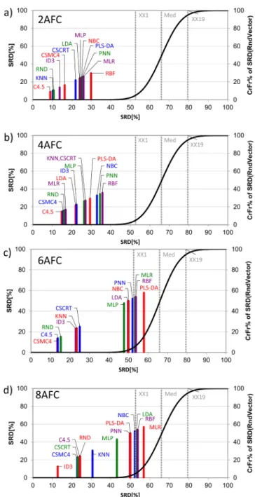
The sum of ranking differences (SRD) provides the rankings of the models for all four choice sets (Fig. 2). Although the figure uses a bar plot to visualize the results, both axes present the same units, the normalized SRD values in percentages. The models are ranked on a 45- degree line are the most similar to the gold standard. A solid black curve gives the relative frequencies of random numbers, e.g. if a model is ranked between the 5% percentile (denoted by XX1 on the plots) and the 95% one (denoted by XX19 on the plots), its ranking cannot be distin- guished from random ranking. All models were placed before XX1 in the case of 2 and 4 alternative forced-choice (AFC); therefore, their ranking is considered significant. The grouping of lines in Fig. 2 (models) suggests a difference in their performances. Decision tree models are grouped together close to zero, which grouping is expressed more as the number of alternatives increases. The superiority of decision trees has been introduced in our earlier study, where only 4AFC tests were analyzed (Gere et al., 2016). On the one hand, the rank of the decision trees shows some variations, and a clear winner cannot unambiguously be defined based on the SRD plots presented in Fig. 2. On the other hand, the superiority of decision trees becomes more expressed as the number of alternatives increases.

A recently introduced validation method to SRD (H´eberger & Koll´ar- Hunek, 2019) enables us to compare the performance of the models more deeply since some influential factors can significantly affect the evaluation of SRDs. The two validation variants of cross-validations are manifested in ANOVA factors and coded by F1, F2 which covers the sampling (F1: two levels: contiguous and resampling without and with replacement, respectively), the number of folds (F2: three levels: fivefold, sevenfold, and tenfold cross-validation) and the third factor (F3) are the models to be compared (F3: 13 levels). In order to be able to find a generally good performing model, the data sets have been merged (e.g.

the four choice sets, each set consisting of four choice tasks) and analyzed as one large data table.

The validation results are presented in Table 1, where factor F3 (the classification models) exhibit highly significant behavior as compared to the theoretically best possible model, as expected. Although the two other factors (the way of cross-validation and number of folds) show no significant effects, their interaction proved to be significant, although the p-value is close to 0.05. The other factors and their interactions show no significant effects as expected and this is reassuring insofar, we have not introduced any bias with resampling (bootstrapping).

ANOVA of Table 2 is visualized in Fig. 3. Although the interaction is significant on the 5% level but not at the 1% level, the observed trend is the same; the bias increases between 5 and 7-folds and then decreases at 10-folds cross-validation. Our findings are in accordance with the literature as it has been shown that “Smaller training set produces bigger prediction errors.” (Efron & Tibshirani, 1995). These results also support the view that we have not introduced any bias with resampling (bootstrapping).

Fig. 4 introduces factor 3 (classifiers). Smaller SRD% values mean less difference from the gold standard. The grouping of the classifiers is still clear; decision trees show lower SRD values compared to the others.

Roughly two large clusters can be observed “good” and “bad ”classifiers or, better to say, recommended and not recommended classifiers for the given task.

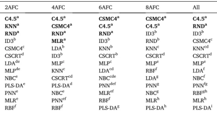
In order to compare the rankings statistically, multiple post hoc tests have been applied (Scheff´e, Tukey-HSD, Bonferroni and LSD); however, all agreed on the homogenous subgroups; therefore only the results of Tukey HSD will be presented in Table 2. Tukey post hoc tests have been run on the four choice sets of separate SRD calculations and on the merged (All) SRD data, as well. C4.5 and CSMC4 proved to be the most reliable method. While C4.5 was ranked as first in the case of a lower number of alternatives (2AFC and 4AFC), CSMC4 showed better performance in the case of 6AFC and 8AFC. However, in the case of the merged data set, C4.5 proved to be better. Possible causes of these

Fig. 2. The SRD values (scaled between 0 and 100) of the performance parameters determined by the sum of ranking differences. An optimum model was used as a reference (benchmark) column, which had the best possible charac- teristics of the performance metrics used. Scaled SRD values are plotted on x axis and left y axis, right y axis shows the relative frequencies of the random ranking distribution function: black curve. Probability levels 5% (XX1), Median (Med), and 95% (XX19) are also given. If a line for a model overlaps the Gauss- curve (XX1) say at p =0.10 then, the method ranks the variable as random with a 10% chance. a) two-alternative forced choice test, b) four-alternative forced- choice test, c) six-alternative forced-choice test, d) eight-alternative forced choice test. Abbreviations: AFC – alternative forced-choice test, KNN - k-nearest neighbor’s, ID3 - Iterative Dichotomiser 3, CSMC4 - Cost-sensitive Decision Tree, C4.5 - Quinlan’s C4.5 decision tree, CSCTR - Cost-sensitive Classification Tree, RND - Random Trees, PLS-DA - Partial Least Squares Discriminant Anal- ysis, LDA - Linear Discriminant Analysis, MLP - Multilayer Perceptron Neural Network, NBC - Naïve Bayes with Continuous variables, RBF - Radial Basis Function Neural Network, PNN - Prototype Nearest Neighbor, MLR - Multino- mial Logistic Regression.

(5)

differences might come from the participants, as significant differences could be observed between participants regarding their mood, emotional state, thinking style et cetera during eye-tracking measure- ments. It has to be mentioned that the best performances were observed in the case of decision trees with one exception. MLR also performed well at 4AFC.

There is an inconsistency between Fig. 2d and Table 2 here. Fig. 2d suggests that ID3 has the most similar performance to the reference (benchmark) column; however, Table 2 shows different results. Results of Table 2 present the rank of the models after cross-validation. The high variance and bias of ID3 during cross-validation made the changes in the ranking.

The superiority of C4.5 model has been identified in other data science studies and has been described as“ a landmark decision tree program that is probably the machine learning workhorse most widely used in practice to date” (Witten, Frank, & Hall, 2011). The obtained results show right consistency since decision trees have been identified in an earlier study conducted by Austrian participants using only 4AFC choice sets (Gere et al., 2016). It must be mentioned that these results should not be generalized, and the authors encourage researchers to test a wide range of classification models before choosing one. It is promising, however, that the SRD algorithm is sensitive to very small differences among the Table 1

Analysis of variance of all models’ SRDs.

Effect SS Df MS F-value p-value

Intercept Fixed 481758.8 1 481758.8 21739.09 <0.001

F1: Contiguous/resampling Random 9.6 1 9.6 5.68 0.099

F2: Fivefold,

sevenfold, and tenfold CV Random 27.9 2 13.9 8.43 0.062

F3: Classifier Fixed 77834.5 12 6486.2 6741.53 <0.001

F1*F2 Random 2.7 2 1.4 4.06 0.030

F1*F3 Random 8.0 12 0.7 1.98 0.074

F2*F3 Random 15.2 24 0.6 1.90 0.062

F1*F2*“F3 Random 8.0 24 0.3 0.05 1.000

Error 3476.3 468 7.4

Abbreviations: CV, cross-validation; MS, mean square residuals; Df, degree of freedom; MS, mean sum of squares; F, Fisher statistics; p, probability of significance; SS, sum of squared residuals. Significant items are indicated by bold.

F1—way of cross-validation (validation variants), two levels: contiguous and resampling. F2—number of folds, three levels: fivefold, sevenfold, and tenfold cross- validation. F3—classifiers to be compared, 13 levels.

Table 2

Tukey post hoc test results (denoted by letters) of the SRD’s.

2AFC 4AFC 6AFC 8AFC All

C4.5â C4.5â CSMC4â CSMC4â C4.5â

KNNâ CSMC4â C4.5â C4.5â RNDâ

RNDâ RNDâ RNDâ ID3^b ID3^b

ID3^b MLR^a ID3^b RND^b CSMC4^c

CSMC4^c LDA^b KNN^b KNN^c KNN^cd

CSCRT^d ID3^b CSCRT^b CSCRT^d CSCRT^d

LDA^de MLP^c MLP^c MLP^e MLP^e

MLP^de KNN^c LDA^cd RBF^f LDA^f

NBC^e CSCRT^cd NBC^cde LDA^g NBC^f

PLS-DA^e PLS-DA^d PNN^def PNN^g PNN^fg

PNNê NBCê MLRêf NBC^g RBF^gh

MLR^e PNN^ef RBF^f MLR^h MLR^h

RBF^f RBF^f PLS-DA^g PLS-DA^h PLS-DAⁱ

Letters in superscript denote the homogenous subgroups determined by Tukey HSD post hoc test after ANOVA. Abbreviations: KNN - k-nearest neighbor neighbor’s, ID3 - Iterative Dichotomiser 3, CSMC4 - Cost-sensitive Decision Tree, C4.5 - Quinlan’s C4.5 decision tree, CSCTR - Cost-sensitive Classification Tree, RND - Random Trees, PLS-DA - Partial Least Squares Discriminant Analysis, LDA - Linear Discriminant Analysis, MLP - Multilayer Perceptron Neural Network, NBC - Naïve Bayes with continuous variables, RBF - Radial Basis Function Neural Network, PNN - Prototype Nearest Neighbor, MLR - Multinomial Logistic Regression, AFC – alternative forced-choice test (numbers before AFC indicate the number of alternatives), All – the merged data set of all AFCs.

Fig. 3. Interaction between factors F1 and F2 (the 5-, 7-, and 10-fold cross- validations done after stratified selection (A, blue lines) and repeated random selection (B, red lines)). (For interpretation of the references to colour in this figure legend, the reader is referred to the web version of this article.)

Fig. 4.Comparison of classifiers. Abbreviations: KNN - k-nearest neighbor- neighbor’s, ID3 - Iterative Dichotomiser 3, CSMC4 - Cost-sensitive Decision Tree, C4.5 - Quinlan’s C4.5 decision tree, CSCTR - Cost-sensitive Classification Tree, RND - Random Trees, PLS-DA - Partial Least Squares Discriminant Anal- ysis, LDA - Linear Discriminant Analysis, MLP - Multilayer Perceptron Neural Network, NBC - Naïve Bayes with Continuous variables, RBF - Radial Basis Function Neural Network, PNN - Prototype Nearest Neighbor, MLR - Multino- mial Logistic Regression.

(6)

performance parameters of the classifiers (H´eberger, 2010; R´acz, Bajusz,

& H´eberger, 2019); therefore, there is a good chance of finding a deci-

sion tree (C4.5 and CSMC4) as the best performing classifier.

Another important aspect of generalization might be cultural differences since visual attention toward food-item images can vary as a function of culture (Zhang & Seo, 2015). However, a recent study introduced that “For foods with higher preference levels, the number of gaze point fixations increased significantly and the total gaze point fixation time significantly increased.” (Yasui, Tanaka, Kakudo, & Tanaka, 2019). Based on these findings, we might propose that prediction models are good tools to predict food choice with a high accuracy using eye-tracking data.

4. Conclusions

Decision trees proved to be superior in all cases, regardless of the choice sets and food product categories. Our validation process proved that C4.5 and CSMC4 decision trees are to be suggested to predict choice based on eye-movements. These results are somewhat deviating since on the one hand, C4.5 showed the best performance at 2AFC, 4AFC, while CSMC4 proved to be the best at 6AFC and 8AFC. On the other hand, C4.5 was defined as best performing with the merged (all choice sets) data set.

Comparing the results to our previous ones (Gere et al., 2016), the joint observation is that decision trees showed the best performance regardless of the number of alternatives. The earlier best ID3 is still ordered into the best four algorithms (see Fig. 2a, c, d). We cannot define a globally best performing method, reasonably, we can suggest decision trees as the best family of classifiers for choice prediction based on eye- movements. As the number of alternatives increases, the judgments become more and more uncertain, SRD values are shifted in the direc- tion of random ranking (c.f. Fig. 2). It is also interesting to observe that CSMC4 models showed better performance in the case of higher numbers of alternatives (6AFC and 8AFC), while C4.5 had the best performance for lower ones (2AFC and 4AFC).

In the presented study, we used default settings of the classification models since fine-tuning was expected to increase overfitting. However, fine-tuning of C4.5 and CSMC4 could help to define the superior one in a given situation. A further future challenge is the application of these models on data from mobile eye-trackers in order to be able to predict choice in more realistic situations.

CRediT authorship contribution statement

Attila Gere: Conceptualization, Methodology, Formal analysis, Investigation, Resources, Writing - original draft, Visualization, Project administration, Funding acquisition. K´aroly H´eberger: Methodology, Validation, Formal analysis, Resources, Data curation, Writing - review

& editing, Visualization, Supervision, Funding acquisition. S´andor

Kovacs: Software, Formal analysis, Data curation, Writing - review ´ &

editing.

Declaration of Competing Interest

The authors declare that they have no known competing financial interests or personal relationships that could have appeared to influence the work reported in this paper.

Acknowledgements

AG thanks the support of the Premium Postdoctoral Researcher Program of the Hungarian Academy of Sciences. The authors thank the support of the National Research, Development, and Innovation Office of Hungary (OTKA, contract No K 134260). This project was supported by the J´anos Bolyai Research Scholarship of the Hungarian Academy of Sciences.

Appendix A. Supplementary material

Supplementary data to this article can be found online at https://doi.

org/10.1016/j.foodres.2021.110309.

References

Bhavsar, H., & Ganatra, A. (2012). A Comparative Study of Training Algorithms for Supervised Machine Learning. International Journal of Soft Computing and Engineering, 2(4), 74–81.

Bialkova, S., Grunert, K. G., & van Trijp, H. (2020). From desktop to supermarket shelf:

Eye-tracking exploration on consumer attention and choice. Food Quality and Preference, 81, Article 103839. https://doi.org/10.1016/j.foodqual.2019.103839.

Bojko, A. (2013). Eye tracking the user experience. Brooklyn, New York: Rosenfeld Media.

Danner, L., de Antoni, N., Gere, A., Sipos, L., Kov´acs, S., & Duerrschmid, K. (2016). Make a choice! Visual attention and choice behavior in multialternative food choice situations. Acta Alimentaria, 45(4), 515–524. https://doi.org/10.1556/

066.2016.1111.

Duda, R. O., Hart, P. E., & Stork, D. G. (2000). Pattern Classification (2nd ed.). Hoboken, New Jersey, NY: Wiley-Interscience.

Duerrschmid, K., & Danner, L. (2018). Eye tracking in consumer research. In G. Ares, &

P. Varela (Eds.), Methods in Consumer Research (Vol. 2, pp. 279–318). https://doi.

org/10.1016/B978-0-08-101743-2.00012-1.

Efron, B., & Tibshirani, R. (1995). Cross-Validation and the Bootstrap: Estimating the Error Rate of a Prediction. In Technical Report No 477.

Fiedler, S., Schulte-Mecklenbeck, M., Renkewitz, F., & Orquin, J. L. (2020). Guideline for Reporting Standards of Eye-tracking Research in Decision Sciences. PsyArXiv, September. https://doi.org/10.31234/osf.io/f6qcy.

Gere, A., Danner, L., de Antoni, N., Kov´acs, S., Dürrschmid, K., & Sipos, L. (2016). Visual attention accompanying food decision process: An alternative approach to choose the best models. Food Quality and Preference, 51. https://doi.org/10.1016/j.

foodqual.2016.01.009.

Gere, A., Danner, L., Dürrschmid, K., K´okai, Z., Sipos, L., Huzsvai, L., & Kov´acs, S. (2020).

Structure of presented stimuli influences gazing behavior and choice. Food Quality and Preference, 83, Article 103915. https://doi.org/10.1016/j.

foodqual.2020.103915.

Gu, Q., Li, Z., & Han, J. (2011). Generalized Fisher score for feature selection. Uncertainty in Artificial Intelligence, 266–273.

H´eberger, K. (2010). Sum of ranking differences compares methods or models fairly.

TrAC - Trends in Analytical Chemistry, 29(1), 101–109. https://doi.org/10.1016/j.

trac.2009.09.009.

H´eberger, K., & Koll´ar-Hunek, K. (2019). Comparison of validation variants by sum of ranking differences and ANOVA. Journal of Chemometrics, 33(6), Article e3104.

https://doi.org/10.1002/cem.3104.

Holmqvist, K., Nystr¨om, M., Andersson, R., & van de Weijer, J. (2011). Eyetracking. A comprehensive guide to methods and measures. Oxford: Oxford University Press.

Jantathai, S., Danner, L., Joechl, M., & Dürrschmid, K. (2013). Gazing behavior, choice and colour of food: Does gazing behavior predict choice? Food Research International, 54(2), 1621–1626. https://doi.org/10.1016/j.foodres.2013.09.050.

Koll´ar-Hunek, K., & H´eberger, K. (2013). Method and model comparison by sum of ranking differences in cases of repeated observations (ties). Chemometrics and Intelligent Laboratory Systems, 127, 139–146. https://doi.org/10.1016/j.

chemolab.2013.06.007.

Kononenko, I., ˇSimec, E., & Robnik-Sikonja, M. (1997). Overcoming the myopia of ˇ inductive learning algorithms with RELIEF. Applied Intelligence, 7(1), 39–55. https://

doi.org/10.1023/A:1008280620621.

Kotsiantis, S. B. (2007). Supervised Machine Learning: A Review of Classification Techniques. Informatica, 31, 249–268.

Kotsiantis, S., Zaharakis, I. D., & Pintelas, P. E. (2006). Machine learning: A review of classification and combining techniques. Artificial Intelligence Review, 26(3), 159–190. https://doi.org/10.1007/s10462-007-9052-3.

Krajbich, I., Armel, C., & Rangel, A. (2010). Visual fixations and the computation and comparison of value in simple choice. Nature Neuroscience, 13(10), 1292–1298.

https://doi.org/10.1038/nn.2635.

Li, C., & Xu, J. (2019). Feature selection with the Fisher score followed by the Maximal Clique Centrality algorithm can accurately identify the hub genes of hepatocellular carcinoma. Scientific Reports, 9, 17283. https://doi.org/10.1038/s41598-019-53471- R´acz, A., Bajusz, D., & H0. ´eberger, K. (2019). Multi-Level Comparison of Machine Learning

Classifiers and Their Performance Metrics. Molecules, 24(15). https://doi.org/

10.3390/molecules24152811.

Rakotomalala, R. (2005). TANAGRA: un logiciel gratuit pour l ’ enseignement et la recherche. In Proceedings of EGC’2005 (Vol. 2, pp. 697–702).

Samant, S. S., & Seo, H. S. (2016). Effects of label understanding level on consumers’

visual attention toward sustainability and process-related label claims found on chicken meat products. Food Quality and Preference, 50, 48–56. https://doi.org/

10.1016/j.foodqual.2016.01.002.

Tobii (2020). Eye tracking study recruitment – managing participants with vision irregularities. Retrieved from https://www.tobiipro.com/blog/eye-tracking-study-re cruitment-managing-participants-with-vision-irregularities/.

Urbanowicz, R. J., Meeker, M., La Cava, W., Olson, R. S., & Moore, J. H. (2018). Relief- based feature selection: Introduction and review. Journal of Biomedical Informatics, 85(July), 189–203. https://doi.org/10.1016/j.jbi.2018.07.014.

(7)

van der Laan, L. N., Hooge, I. T. C., De Ridder, D. T. D., Viergever, M. A., &

Smeets, P. A. M. (2015). Do you like what you see? The role of first fixation and total fixation duration in consumer choice. Food Quality and Preference, 39, 46–55.

https://doi.org/10.1016/j.foodqual.2014.06.015.

Witten, I. H., Frank, E., & Hall, M. A. (2011). Chapter 6 - Implementations: Real Machine Learning Schemes. In Ian H. Witten, Eibe Frank and Mark A. Hall (Eds.), The Morgan Kaufmann Series in Data Management Systems (pp. 191–304). https://doi.org/10.10

16/B978-0-12-374856-0.00006-7. https://www.sciencedirect.com/book/9780 123748560/data-mining-practical-machine-learning-tools-and-techniques.

Yasui, Y., Tanaka, J., Kakudo, M., & Tanaka, M. (2019). Relationship between preference and gaze in modified food using eye tracker. Journal of Prosthodontic Research, 63(2), 210–215. https://doi.org/10.1016/j.jpor.2018.11.011.

Zhang, B., & Seo, H.-S. (2015). Visual attention toward food-item images can vary as a function of background saliency and culture: An eye-tracking study. Food Quality and Preference, 41, 172–179. https://doi.org/10.1016/j.foodqual.2014.12.004.