The efficiency of classification in imperfect databases: Comparing kNN and correlation clustering

The efficiency of classification in imperfect databases: comparing kNN and correlation

clustering

Mária Bakó

University of Debrecen Faculty of Economics and Business

bakom@unideb.hu

Submitted June 5, 2018 — Accepted August 10, 2018

Abstract

In every day life it is usually too expensive or simply not possible to determine every attribute of an object. So for example, it would not come as a surprise that hospitals only conduct a CT or MRI in given circumstances.

Hence it is quite a common problem at such classifications, that data is lacking for both the objects forming the existing classes and the objects needing to be sorted. There exist different algorithms that try to make up the missing information and do the calculations for the classification based on these, and there are also some algorithms that only use the existing data and nothing else. In this article we compare two algorithms, the well-known kNN and one based on correlation clustering. Whilst the former only extrapolates based on accessible data, the latter only uses existing data.

Keywords:classification, kNN, missing data, correlation clustering MSC:68W20, 62H30, 91C20

1. Introduction

Data mining aims to extract important but not yet established information from databases. For the different types of questions we used a variety of algorithms.

From these the most important two are classification and clustering.

doi: 10.33039/ami.2018.08.002 http://ami.uni-eszterhazy.hu

11

• Classification, here, we are given a grouping and we need to decide for each new object which class it would best fit into. For example, a lecturer would know how to grade students based on their results. In case of a new exam, they would be able to give fair marks based on their previous experience of marking exams. There are different way to classify something:

– decision trees, for each leaf there is a matching class, and for every question asked at a node, the answers direct the path forward. At the end of the path we are given the class of the object we are classifying [12].

– Bayes-classification, by creating a model we get a Bayes-network with corresponding conditional probabilities. From these it is possible to de- termine the probability distribution of an object’s relation to the classes, and so it is possible to classify the object accordingly [11]. This is how spam mail is filtered as well.

– neural networks, through the learning process, the edges of the neural network are assigned corresponding weights. Then, by entering the ob- ject parameters as the input variable, the output variables automatically present the weighting of the different classes [10].

– knearest neighbour (or kNN) here, using the original classification, we need to determine theknearest neighbour for the objects needing to be classified, and from these the most commonly occurring one gives the class of the object [6].

– fuzzy classifier, in this case we have membership functions, in the form of if. . . , then. . . fuzzy rules which generate a fuzzy set for each class from which, using the attributes of the object given as an input, the most accurate classification can be made [9].

• In case ofclustering, the grouping of objects is not known, hence the classes do not exists and need to be constructed. A large number of algorithms have been created and almost all of them uses the distances between objects. Here, we actually use an algorithm that does not build directly on distances, hence we avoid presenting the distance based ones.

In the next chapter we present the details and refinement of kNN, so that we can use this algorithm even when data might be missing. Then we present correlation clustering and the classification methods that are built on it. Then using our numerical results we demonstrate the two methods using a concrete example. Following the discussion, we collect the results and explore possible further research paths.

2. Refining the kNN method

2.1. Distances

The k nearest neighbour algorithm is built on distances. Hence we investigate distances a bit further. The data is usually described by ann-tuple. This sometimes only contains numbers, which describe quantities instead of any code. In this case thisnnumbers can be perceived as a point in then-dimensional space. To evaluate the distance between two such points we use the Minkowski-distance:

d(p, q) =Xⁿ

i=1

|pi−qi|^m_m¹ ,

which in special cases gives the Manhattan (m= 1), Eucledian (m= 2) or Cheby- shev (m=∞) distance.

If one of the points from then-dimensional space is missing a coordinate then it could be positioned anywhere on a straight line, hence its distance from another point could be anything from a hyperplane distance inn−1 dimension to infinity.

Hence it could be considered reckless to replace the missing coordinate with a concrete value, which has 0probability to be accurate.

However, when describing humans, we measure height in meters and weight in kilograms

• if two people have the same weight but one is 1 meter higher than the other, we consider them to be completely different, whilst

• if two people have the same height and differ in weight by 1 kilogram, then they can be considered very similar.

Hence it is worth normalising the data. Since the data used in testing comes from real-life, we assume that the different dimensions have normal distribution and hence the transformation brought us into ann-dimensional normal distribution.

2.2. Supplementing data

One of the most commonly used method for supplementing data is to replace the missing term with the average of the other data, and this is directly stored in the database hence once the replacement is done, the artificially constructed data cannot be differentiated from the original. If data is missing from a learning object, then we could simply just take the average of the objects corresponding to its coordinates. However, if data is missing from an object to be classified, we do not know which class it would belong to, hence it is best to use the average of all objects.

Since we wish to compare two algorithms on the same learning objects and objects to be classified, we need to find a better way to substitute the missing data. As the Minkowski distance is based on coordinate-wise distances|pi−qi|, we

will have some missing values. Hence we calculate the the average of the existing ones: d¯=P

i|pi−qi|/l, wherel is the number of existing distances. Therefore we now work with an estimated distance instead of the concrete ones.

d⁰(p, q) = X

i

|pi−qi|^m+ (n−l) ¯d^m_m¹ .

2.3. Considering reliability

The original kNN algorithm aims to determine such an environment for every learning object where there are exactlykclassified objects. Then for every class it determines the prevalence and chooses the class that occurs the most. Note, that it does not make any difference based on which classified object is the closest (i.e.

is the most similar) to the learning object.

Suggestions have been made to create a weighting system [8], which punishes the neighbours that are further away. However this does not consider the fact that neighbouring could have followed directly from the original, or equivalently, the made up data.

In our implementation we combine these two viewpoints and multiply the dis- tance of two points byn/l(1 +d⁰), whered⁰ is the estimated distance, andlout of nis the number of dimensions where two objects can be compared. As this number gets smaller, the weight grows, the weighed distance grows and so the value will be considered less and less.

The weighed distances were ordered and theksmallest ones were summarised based on their classes. It is possible that the learning and classified objects both have some available data, but not in the same dimensions, so the average distance d¯cannot be calculated. We omit these cases.

3. Correlation clustering

3.1. Basic concepts

The aim of clustering is to partition the set of objects in such a way that the similar objects are in the same subset, and dissimilar objects are in different subsets.

Even if given a similarity relation it may not be possible to create such a par- tition where this holds for every pair of elements. For example, consider the set of whole numbers, where two numbers are dissimilar is they are coprime. Here 4and6are similar, as well as6and9, however4and9are dissimilar. Such a sim- ilarity relation, that is reflexive, symmetric but not necessarily transitive is called a tolerance relation.

The aim of correlation clustering is to provide theclosest equivalence relation to a given tolerance relation [13]. The distance of the two relations is given by the number of pairs that are similar but in different subsets, or dissimilar and in the same subset.

Solving a correlation clustering is NP-hard, hence typically we can only use approximating algorithms to find a near optimal solution [5].

3.2. Method of contractions

The aim of correlation clustering can also be considered as an optimisation prob- lem. Hence we can accordingly use optimisation methods on it. However our measurements show that these do not yield satisfying results [1, 4]. Hence we have implemented the method of contractions, which models the behaviour of charged particles or magnetic materials. We start with a partition of the base set containing only singletons, and we merge the clusters that attract each other. Attraction of a cluster is the superposition of attraction of its elements. We obviously need to check whether any of the clusters rejects any of its elements, since if it does then we need to create a new singleton containing that element. We continue this until the whole system becomes stable. In case of stability, these clusters form the partition.

3.3. Generating a tolerance relation

Correlation clustering itself requires a tolerance relation, however this is available only for a few clustering problems. From the raw data we can only hope to gain information about the distances. Therefore if we wish to use our method in more cases then we need to construct a tolerance relation out of these distances.

For constructing a clustering based on distance, if two points are close enough to each other then we treat them as similar and if they far away from each other we treat them as dissimilar. Therefore we introduce two constants (δand ∆), which represent similarity and dissimilarity, respectively. Two objects not being similar does not necessarily mean dissimilarity, since in that case it would be enough to introduce a single constant. This may be simple in some cases, like at our previous example based on coprimes. However, in real life there are numerous cases where two objects are not or simply cannot be compared. Then we are met with partiality, that is, neither of the relations hold.

It would be easy to assume that if the distance of two objects is below the given smaller limit then they are similar, if above the other then dissimilar, and otherwise neither.

Whilst this would be a plausible interpretation, we chose a more general method, we use two distance functions (f andF). One defines similarity and the other the difference. So then if F(p, q) > ∆ then two objects are considered dissimilar.

Similarly, if f(p, q) < δ then two objects are similar. If none of these hold then there is no relation between them. Hence from here on it is possible to generate a tolerance relation using hδ,∆, f, Fi. Now we need to determine which will be the most useful for our requirements.

3.4. Classification using correlation clustering

Quite often with correlation clustering there are more than one (near) optimal solutions. We could create an intersection out of the different partitions, however it is impossible to tell apart the elements of the resulting P partition. Therefore using rough set theory terminology, we consider these elements indistinguishable.

SoP defines a Pawlakian base set system.

This gives us the option to create a rought set theory approximation for the classification of the set of those objects. The subsets of P are associated with classes based on which class’ elements are the most popular inside of them [2].

This concludes the learning needed for the classification, and we can start allo- cating the elements that need to be classified into classes. Now we are interested in how much the elements of the base set (i.e. the elements of the partition) attracts or rejects the new object. We add the new object to the most favourable cluster.

We could use soft-classification, and we could classify the new object based on the proportion of the classes of elements in the cluster, but we chose a more clear-cut approach instead. Hence if there is a tie within a cluster (two classes have the same number of objects) then we do not classify the object.

We need to consider whether the other clusters could be helpful, i.e. whether we could superposition the attraction of all the clusters corresponding to a given class.

Whilst this should be technically doable, it usually ends in questionable results as seen later in the discussion.

3.5. Handling imperfect data

Given two object, both possibly missing some data. We could not fully call them similar since the missing data may be hiding critical dissimilarity. So the missing data may suggest a bigger distance. If two objects are considered dissimilar even the missing data would not change that.

Traditionally for partial tolerance relations we symbolise the three different possibilities with the numbers {−1,0,1}, which represent that two object are dis- similar, not comparable and similar, respectively.

In case of missing data, similarity and certainty are symbolised with a number between [−1,1]. The closer it is to either endpoint the more certain the decision becomes [3]. Following the above, the value of the tolerance relation (t(p, q)) for objectspandqis:

• if the two objects are definitely dissimilar (F(p, q)>∆), thent(p, q) =−1,

• if the two object are different when we extrapolate their distance (F(p, q)>

∆·l/n, but F(p, q) < ∆), then t(p, q) = −l/n, where l is the number of comparable dimensions.

• if the two objects are similar when extrapolate their distance (f(p, q)< δ·l/n andF(p, q)<∆·l/n), thent(p, q) =l/n

• and in every other caset(p, q) = 0.

Interestingly, the method of contraction for generalised tolerance relation wor- ked without any changes. Due to the nature of the algorithm, first it merges the objects without any missing data and only when these are all done can the objects with missing data be processed. Then the creation of the intersection of partitions ofP is done exactly as above.

4. Discussing our results

From the UCI Machine Learning Repository we chose the Wine Data Set for test- ing [7]. This contains 178 italian wines, which can be described by 13 chemi- cal/physical traits. The wines can be sorted into3categories. For the learning set we obviously use this information, whilst for the other wines we check whether the classification put them into the right classes.

For our experiments we randomly selected 25 wines into each learning sets.

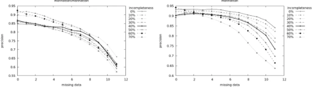
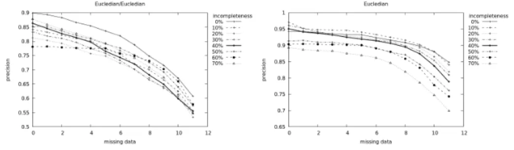
Since we would like to inspect the effect of the missing data for both methods, in 7steps we managed to randomly delete5%of data. Hence we lose information for both the original sample and the wines to be classified. The different stages of the learning sets are marked with dashed lines.

Additionally, for every wine to be classified we deleted1 piece of information 11 times. This is represented on the horizontal axis. The vertical axis represents the rate at which we managed to correctly guess the category of the wine.

We generated a100 learning sets and step by step we deleted data from them similarly to the elements awaiting classification.

We conducted these experiments for each of distance types we have introduced above, and in case of correlation clustering for all pairs of distances as well.

Figure 1: Using Manhattan distance

On Figures 1–3 we can see that the Chebyshev distance yielded the worst result.

Interestingly, sometimes it is better to have less data. This is likely related to the fact that in a uniform sphere in this case (due to maximal distance) a cube, the objects placed at the nodes may seem to be different and may be considered to be part of this class by mistake. Looking at the graphs on the left, and considering Euclidian and Manhattan distances, the recognition rate of objects to be classified decreases evenly until about half the amount of data is deleted and then the slope

Figure 2: Using Euclidian distance

Figure 3: Using Chebishev approximation

Figure 4: Using attraction of lower approximations

changes. Looking at the graphs on the right, where we used kNN, the recognition rate does not change much until about half the amount of data is deleted, however afterwards the deletion makes a big difference.

On Figures 1–3 we can see a variant where the object to be classified is added to the most attractive cluster. On Figure 4, we focused on the attraction of the lower approximation of classes. From these graphs we can see that this approximation is not the most rewarding. The original classification of the learning elements is an artificial creation, and it does not show the potential sub-classes. Since correlation clustering aims for optimisation and finding the minimal distance from an equivalence relation, which may happen in multiple different way, it finds a refinement of the original classification. This is facilitated by favouring the base set system, which is the closest to the original classification - that is, the least number of base sets belong to more than one class of the learning set.

We can also inspect the effect ofk on the efficiency of kNN.

5. Conclusion and future research direction

We have presented a classification method alongside the well known kNN that determines its own parameters adaptively, and creates a partition based on these that enables clustering. Determining the parameters and the construction the system of the base set is calculation heavy, and so it scales badly. However it only uses the existing data and so it cannot manipulate them arbitrarily. We use these two methods for the Wine database.

It has been proved again that the widely taught kNN method deserves its fame.

It has given great results even in cases where there was almost no data available for classification purposes.

The method based on correlation clustering could not overpower kNN in any way. However we have only used it for normally distributed data. Hence it would be worth trying out databases where discrete or categorical data are more present to see whether the generated distances would be more useful than the tolerance relations based on the data.

References

[1] Aszalós, L., and Bakó, M. Advanced search methods (in Hungarian). https:

//gyires.inf.unideb.hu/GyBITT/13/, 2012.

[2] Aszalós, L., and Mihálydeák, T. Rough classification based on correlation clus- tering. InRough Sets and Knowledge Technology. Springer, 2014, pp. 399–410.

https://doi.org/10.1007/978-3-319-11740-9_37

[3] Aszalós, L., and Mihálydeák, T. Rough classification in incomplete databases by correlation clustering. InIFSA-EUSFLAT (2015).

[4] Bakó, M., and Aszalós, L. Combinatorial optimization methods for correlation clustering. InCoping with complexity, D. Dumitrescu, R. I. Lung, and L. Cremene, Eds. Casa Cartii de Stiinta, Cluj-Napoca, 2011, pp. 2–12.

[5] Bansal, N., Blum, A., and Chawla, S.Correlation clustering.Machine Learning 56, 1-3 (2004), 89–113.

https://doi.org/10.1023/b:mach.0000033116.57574.95

[6] Bhatia, N., et al. Survey of nearest neighbor techniques. arXiv preprint arXiv:1007.0085 (2010).

[7] Dheeru, D., and Karra Taniskidou, E. UCI machine learning repository, 2017.

[8] Dudani, S. A. The distance-weighted k-nearest-neighbor rule. IEEE Transactions on Systems, Man, and Cybernetics, 4 (1976), 325–327.

https://doi.org/10.1109/tsmc.1976.5408784

[9] Ishibuchi, H., Nozaki, K., Yamamoto, N., and Tanaka, H. Selecting fuzzy if-then rules for classification problems using genetic algorithms.IEEE Transactions on fuzzy systems 3, 3 (1995), 260–270.

https://doi.org/10.1109/91.413232

[10] Lippmann, R.An introduction to computing with neural nets.IEEE Assp magazine 4, 2 (1987), 4–22.

https://doi.org/10.1109/massp.1987.1165576

[11] Mosteller, F., and Wallace, D. L. Applied Bayesian and classical inference:

the case of the Federalist papers. Springer Science & Business Media, 2012.

[12] Quinlan, J. R. Induction of decision trees. Machine learning 1, 1 (1986), 81–106.

https://doi.org/10.1007/bf00116251

[13] Zahn, Jr, C. Approximating symmetric relations by equivalence relations. Journal of the Society for Industrial & Applied Mathematics 12, 4 (1964), 840–847.

https://doi.org/10.1137/0112071