Field dependence of the Yukawa coupling in the three flavor quark–meson model G. Fej˝os

Field dependence of the Yukawa coupling in the three flavor quark–meson model

G. Fej˝os^∗ and A. Patk´os^†

Institute of Physics, E¨otv¨os University, 1117 Budapest, Hungary

We investigate the renormalization group flow of the field-dependent Yukawa coupling in the framework of the three flavor quark–meson model. In a conventional perturbative calculation, given that the field rescaling is trivial, the Yukawa coupling does not get renormalized at the one-loop level if it is coupled to an equal number of scalar and pseudoscalar fields. Its field-dependent version, however, does flow with respect to the scale. Using the functional renormalization group technique, we show that it is highly nontrivial how to extract the actual flow of the Yukawa coupling as there are several new chirally invariant operators that get generated by quantum fluctuations in the effective action, which need to be distinguished from that of the Yukawa interaction.

I. INTRODUCTION

One of the merits of the functional renormalization group (FRG) technique is that it allows for calculating the flows of n-point functions nonperturbatively. Via the FRG one has the freedom to evaluate the scale depen- dence of them in nonzero background field configurations, which is thought to be essential once spontaneous sym- metry breaking occurs [1–3]. For the sake of an example, in scalar (φ) theories, quantum corrections to the wave function renormalization (Z) typically vanish at the one- loop level, but using the FRG one gets a nonzero con- tribution once one generalizes the corresponding kinetic term in the effective action as∼Z(φ)∂µφ∂^µφ and eval- uates Z at a symmetry breaking stationary point of the effective action. This procedure is essential, e.g., in two- dimensional systems that undergo topological phase tran- sitions, as the wave function renormalization is known to be diverging in the low temperature phase, which cannot be described in terms of perturbation theory [4]. Simi- larly, in four dimensions, it has recently been shown that in the three flavor linear sigma model the coefficient of ‘t Hooft’s determinant term also receives substantial con- tributions when evaluated at nonzero field [5].

A similar treatment should be in order for Yukawa in- teractions, whose renormalization group flow vanishes at the one loop level, if complex scalar fields are coupled to the fermions and the field strength renormalization is trivial [6]. In phenomenological investigations of the two and three flavor quark–meson models several pa- pers have dealt with the nonperturbative renormaliza- tion of the Yukawa coupling. The essence of the corre- sponding calculations is that one determines the RG flow of the fermion–fermion–meson proper vertex, defined as δ³Γ/δLψδ¯ Rψδφin a given background (Γ being the effec- tive action), and then associates it with the flow of the Yukawa coupling itself. This obviously works for one fla- vor models [7, 8], and even for the two flavor case [9, 10], in particular for models restricted to theσ−πsubsector, i.e., withO(4) symmetry in the meson part of the theory.

∗gergely.fejos@ttk.elte.hu

†patkos@galaxy.elte.hu

The reason why the approach has legitimacy in the latter case is that it turns out that the only way fluctuations generate new Yukawa–like operators in the quantum ef- fective action is that the original Yukawa term is mul- tiplied by powers of the quadraticO(4) invariant of the meson fields. That is to say, one is allowed to choose, e.g., a vacuum expectation value for which all pseudoscalar (π) fields vanish, but the scalar (s) one is nonzero, and associate∼s² with the aforementioned quadratic invari- ant leading to the appropriate determination of the field dependence of the Yukawa coupling.

The situation is not that simple in case of three fla- vors, i.e., chiral symmetry of U_L(3)×U_R(3). Since the effective action automatically respects linearly realized symmetries of the Lagrangian, field dependence of any coupling must mean all possible functional dependence on chirally invariant operators. Because there are more invariants compared to the two flavor case, if one chooses a specific background for the evaluation of the RG flow of the fermion–fermion–meson vertex, one may arrive at an “effective” Yukawa interaction, but it will then mix in that specific background the contribution of different chirally invariant operators. The reason is that for three flavors other operators than that of the Yukawa term (multiplied by powers of the quadratic invariant) can get generated, which are presumably not even considered nei- ther in the Lagrangian nor in the ansatz of the effective action. The newly emerging operators in principle can- not be distinguished from the Yukawa interaction if the background is too simple, and as it will be shown, a naive calculation squeezes inappropriate terms into the Yukawa flow, which should be separated via the choice of a suit- able background and projected out.

Investigations of the three flavor case including the ef- fects of the U_A(1) anomaly were started by Mitter and Schaefer. In a first paper, no RG evolution of the Yukawa coupling was taken into account [11]. This approxima- tion was carried over in several directions, including in- vestigations regarding magnetic [12] and topological [13]

susceptibilities, mass dependence of the chiral transition [14], or quark stars [15].

A strategy for extracting the RG flow of the field- dependent Yukawa coupling was presented by Pawlowski and Rennecke, explicitly realized for the two flavor case

arXiv:2011.08387v3 [hep-ph] 13 Apr 2021

[10]. In this paper, interaction vertices arising from the expansion of the field-dependent Yukawa coupling were also analyzed and it was found that higher order mesonic interactions to two quarks are gradually less important.

These results were further used in recent ambitious com- putations of the meson spectra from effective models di- rectly matched to QCD [16, 17]. The method of [10]

was then applied for extracting the flow of the Yukawa coupling in the 2+1 flavor (realistic) quark–meson model [18]. The prescription used in the latter calculation re- lies on a symmetry breaking background, from which a field independent Yukawa coupling is extracted. A simi- lar approach has already been introduced in the seminal paper of Jungnickel and Wetterich [19], where a diago- nal symmetry breaking background was employed in cal- culating the RG equation of the Yukawa coupling (for general number of flavors). As a generalization, here we offer a renormalization procedure of the field-dependent Yukawa coupling realizable in any symmetry breaking background through a chirally invariant set of operators.

More specifically, the aim of this paper is to show how to separate the field-dependent Yukawa interaction from those new fermion–fermion–multimeson couplings that unavoidably arise as three flavor chiral symmetry allows for a much larger set of operators in the infrared than considering only a field-dependent Yukawa coupling. For this, the right-hand side (rhs) of the evolution equation of the effective action will be evaluated in such a back- ground that allows for expressing it in terms of explicitly invariant operators, as it was demonstrated for purely mesonic theories some time ago [20–23]. We also note that apart from the above applications, recent studies on a lower Higgs mass bound [24] and on quantum criticality [25] also deal with field-dependent Yukawa interactions.

The paper is organized as follows. In Sec. II, we present the model emphasizing its symmetry properties.

We explicitly show what kind of new operators can be generated and set an ansatz for the scale-dependent effec- tive action accordingly. Section III contains the explicit calculation of the flows generated by the field-dependent Yukawa coupling, and Sec. IV is devoted to an extended scenario where at the lowest order the newly established operators are also taken into account. In Sec. V, we present numerical evidence for the relevance of the pro- posed procedure, while the reader finds the summary in Sec. VI.

II. MODEL AND SYMMETRY PROPERTIES We are working with the U_A(1) anomaly free three flavor quark–meson model, which is defined through the following Euclidean Lagrangian:

L= Tr (∂iM^†∂iM) +m²Tr (M^†M) + ¯λ1 Tr (M^†M)²

+ ¯λ2Tr (M^†M M^†M)

+ ¯q(∂/+gM5)q, (1)

whereM stands for the meson fields,M = (s_a+iπ_a)T_a (Ta = λa/2 are generators of U(3) with λa being the Gell-Mann matrices, a = 0...8), q^T = (u d s) are the quarks, andM5 = (sa+iπaγ5)Ta. As usual, m² is the mass parameter and ¯λ1, ¯λ2 refer to independent quartic couplings. The fermion part contains ∂/ ≡ ∂_iγ_i, γ₅ = iγ₀γ₁γ₂γ₃ with {γi} being the Dirac matrices and the Yukawa coupling is denoted byg.

Concerning the meson fields,UL(3)×UR(3)'UV(3)× UA(3) chiral symmetry manifests itself as

M →V M V^†, M →A^†M A^† (2) for vector and axialvector transformations, respectively, V = exp(iθ^a_VT_a),A= exp(iθ_A^aT_a). This also implies that M₅→V M₅V^†, M₅→A^†₅M₅A^†₅, (3) whereA₅= exp(iθ_A^aT_aγ₅). As for the quarks, the trans- formation properties are

q→V q, q→A5q. (4) Note that, since{γi, γ5}= 0,

¯

q→qV¯ ^†, q¯→qA¯ 5. (5) These transformation properties guarantee that all terms in (1) are invariant under vector and axialvector trans- formations.

The quantum effective action, Γ, built upon the the- ory defined in (1) also has to respect chiral symmetry.

That is to say, only chirally invariant combinations of the fields can emerge in Γ. For three flavors, there exist three independent invariants made out of theM fields,

ρ:= Tr (M^†M),

τ:= Tr (M^†M−Tr (M^†M)/3)²,

ρ3:= Tr (M^†M−Tr (M^†M)/3)³, (6) where the last one is absent in (1) due to perturbative UV renormalizability but nothing prevents its generation in the infrared. In principle, the chiral effective potential, V, defined via homogeneous field configurations, Γ|_hom = R

xV has to be of the form V =V(ρ, τ, ρ₃). Obviously, the generalized Yukawa term,

g(ρ, τ, ρ3)·qM¯ 5q (7) can (and does) also appear in Γ, but in this paper we restrict ourselves to

g(ρ, τ, ρ3)≈g(ρ). (8) This is motivated from a symmetry breaking point of view, i.e., without explicit symmetry breaking terms in (1), chiral symmetry breaks asU_L(3)×U_R(3)→U_V(3) [26], and for any background field respecting vector sym- metries,τ ≡0≡ρ3. We can think of g(ρ) as

g(ρ) =

∞

X

n=0

gnρⁿ= (g0+g1·ρ+...), (9)

which shows that it actually resums operators of the form

∼[ Tr (M^†M)]ⁿqM¯ 5q.

Note that, however, as announced in the Introduction, there are several other invariant combinations at a given order that are allowed by chiral symmetry and contribute to quark–meson interactions. Take the lowest nontrivial order, i.e., dimension 6. We have two invariant combina- tions:

∼ρ·qM¯ 5q, ∼qM¯ 5M₅^†M5q. (10) Obviously the first one is to be incorporated into the field-dependent Yukawa coupling, but not the second one.

Note that one may think of the fifth Dirac matrix as the difference between left- and right-handed projectors, γ5 = PR−PL, and therefore, e.g., the first expression is equivalent to ¯qLM qR+ ¯qRM^†qL and the second to

¯

qLM M^†M qR+ ¯qRM^†M M^†qL. Thus, one can trade the M₅ dependence to M dependence in the invariants via working with left- and right-handed quarks separately.

Going to next-to-leading order, we see the emergence of the following new terms [note that for general configura- tions Tr (M₅^†M5) = Tr (M^†M)]:

∼ρ²·qM¯ ₅q, ∼ρ·qM¯ ₅M₅^†M₅q, ∼qM¯ ₅M₅^†M₅M₅^†M₅q, (11) and we might even have∼τ·qM¯ 5q, though we intend to drop such contributions, see approximation (8). If we are to extract the renormalization group flow of g(ρ), then we need a strategy to distinguish each operator at a given order, in order to be able to resum only the Yukawa inter- actions, and not the aforementioned new quark–quark–

multimeson operators. Obviously, this procedure cannot be done through a one component background field, e.g., the vectorlike condensate M ∼ s₀·1, as it mixes up the corresponding operators, and one loses the chance to recombine the field dependence into actual invariant tensors.

The flow of the effective action is described by the Wet- terich equation [27, 28]

∂kΓk = 1 2 Z

Tr [(Γ⁽²⁾_k +Rk)⁻¹∂kRk], (12) where Γ⁽²⁾_k is the second functional derivative matrix of Γk and Rk is the regulator function. One typically chooses it to be diagonal in momentum space, and set Rk asRk(p, q) = (2π)⁴R_k(q)δ(q+p). Evaluating (12) in Fourier space leads to

∂_kΓ_k= 1 2

Z

p

Tr [(Γ⁽²⁾_k +R_k)⁻¹(p,−p)∂_kR_k(p)].(13) In this paper, the equation will be evaluated only in spacetime-independent background fields; therefore, one assumes that Γ⁽²⁾_k is also diagonal in momentum space, Γ⁽²⁾_k (p, q) = (2π)⁴Γ⁽²⁾_k (q)δ(q+p). In such backgrounds, it

is sufficient to work with the effective potential, V_k, via Γk|hom=R

xVk, and (13) leads to

∂kVk =1 2

Z

p

Tr{(Γ⁽²⁾_k (pR))⁻¹∂kRk(p)}, (14) where we have assumed that the regulator matrix Rk

is meant to replace everywhere pwith p_R, where p_R is the regulated momentum through the R_k function, i.e., p²_R=p²+Rk(p),pRi=pRpˆi.

The ansatz we choose for Γkis called the local potential approximation, which consists of the usual kinetic terms and a local potential (in this case, specifically, a mesonic potential plus the Yukawa term),

Γk= Z

x

h

Tr (∂iM^†∂iM) + ¯q /∂q

+Vch,k(ρ, τ, ρ3) +gk(ρ)¯qM5qi

. (15)

Using the earlier notation,Vk=Vch,k+gk(ρ)¯qM5q. Note that the chiral potential will not be considered in its full generality, but rather asVch,k=Uk(ρ) +Ck(ρ)τ. Flows ofUk andCk can be found in [23]. Note that this con- struction could be easily extended with ‘t Hooft’s deter- minant term describing theU_A(1) anomaly,∼(detM + detM^†), and the corresponding coefficient function. In- vestigations in this direction are beyond the scope of this paper.

III. FLOW OF THE FIELD-DEPENDENT YUKAWA COUPLING

In this section, we evaluate (13) in homogeneous back- ground fields to obtain the flow ofgk(ρ), defined in (15).

Calculating Γ⁽²⁾_k using the ansatz (15), one gets the fol- lowing hypermatrix in the {s^a, π^a, ¯q^T, q} multicompo- nent space:











p²+m²_s,k m²_sπ,k −(~g_k^(s)q)^T q~¯g^(s)_k m²_πs,k p²+m²_π,k −(~g_k^(π)q)^T q~¯g^(π)_k

~

g_k^(s)q ~g^(π)_k q 0 i/p+gkM5

−(¯q~g^(s)_k )^T −(¯q~g_k^(π))^T −i/p−g_kM₅ 0









 ,

(16) where (g_k^(s))a = gk(ρ)Ta + g_k⁰(ρ)saM5, (g^(π)_k )a = igk(ρ)Taγ5+g_k⁰(ρ)πaM5, and the mass matrices are de- fined through the following relations:

(m²_s,k)_ij =∂²V_k/∂s_i∂s_j, (m²_π,k)_ij =∂²V_k/∂π_i∂π_j, (m²_sπ,k)ij =∂²Vk/∂si∂πj. (17) For practical purposes, it is worth to separate Γ⁽²⁾_k into three parts [29, 30], Γ⁽²⁾_k = Γ⁽²⁾_k,B+ Γ⁽²⁾_k,F + Γ⁽²⁾_k,mix, where the respective terms are defined as

Γ⁽²⁾_k,B=









p²+m²_s,k m²_sπ,k 0 0 m²_πs,k p²+m²_π,k 0 0

0 0 0 0

0 0 0 0









, Γ⁽²⁾_k,F =









0 0 0 0

0 0 0 0

0 0 0 i/p+gkM5

0 0 −i/p−g_kM₅ 0







 ,

Γ⁽²⁾_k,mix ≡ 0 Γ⁽²⁾_{k,F B} Γ⁽²⁾_k,BF 0

!

=











0 0 −(~g_k^(s)q)^T q~¯g^(s)_k 0 0 −(~g_k^(π)q)^T q~¯g_k^(π)

~g_k^(s)q ~g_k^(π)q 0 0

−(¯q~g_k^(s))^T −(¯q~g^(π)_k )^T 0 0











. (18)

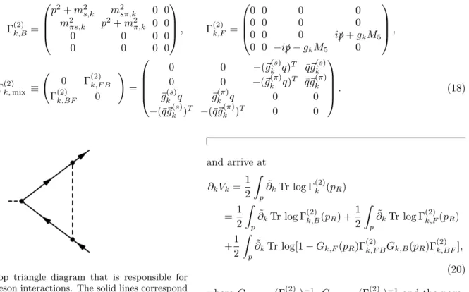
FIG. 1. One-loop triangle diagram that is responsible for flowing quark–meson interactions. The solid lines correspond to quarks, while the dashed ones represent mesons.

FIG. 2. One-loop tadpole diagram arising from the field- dependent Yukawa interaction, which allows the generation of new quark–meson vertices in the RG flow. The solid lines correspond to quarks, while the dashed ones represent mesons.

Using these notations, and by introducing the differential operator ˜∂_k, which, by definition acts only on the regula- tor function,R_k, (14) can be conveniently reformulated.

We may use the matrix identity

Γ⁽²⁾_k,B Γ⁽²⁾_k,BF Γ⁽²⁾_{k,F B} Γ⁽²⁾_k,F

!

= Γ⁽²⁾_k,B 0 Γ⁽²⁾_{k,F B} 1

! 1 (Γ⁽²⁾_k,B)⁻¹Γ⁽²⁾_k,BF 0 Γ⁽²⁾_k,F −Γ⁽²⁾_{k,F B}(Γ⁽²⁾_k,B)⁻¹Γ⁽²⁾_k,BF

!

(19)

and arrive at

∂kVk =1 2

Z

p

∂˜kTr log Γ⁽²⁾_k (pR)

= 1 2 Z

p

∂˜kTr log Γ⁽²⁾_k,B(pR) +1 2 Z

p

∂˜kTr log Γ⁽²⁾_k,F(pR) +1

2 Z

p

∂˜kTr log[1−Gk,F(pR)Γ⁽²⁾_{k,F B}Gk,B(pR)Γ⁽²⁾_k,BF], (20) whereGk,B = (Γ⁽²⁾_k,B)⁻¹, Gk,F = (Γ⁽²⁾_k,F)⁻¹ and the nega- tive sign of the pure fermionic term is understood. We are interested in the flow of the Yukawa coupling; thus, we need to identify in the rhs of (20) the operator∼qM¯ ₅q.

This is in part generated from the leading term of the last contribution of the rhs of (20),

−1 2

Z

p

∂˜_kTr[G_k,F(p_R)Γ⁽²⁾_{k,F B}G_k,B(p_R)Γ⁽²⁾_k,BF]. (21) More specifically, it reads

−¯q Z

p

∂˜k

n

(g_k^(s))aS(pR)G^ab_k,s(pR)(g^(s)_k )b

+(g_k^(π))aS(pR)G^ab_k,π(pR)(g^(π)_k )b

+(g_k^(s))_aS(p_R)G^ab_k,sπ(p_R)(g^(π)_k )_b +(g_k^(π))aS(pR)G^ab_k,πs(pR)(g^(s)_k )b

o

q, (22) where S_k(p) = (i/p+g_kM₅)⁻¹ is the fermion propaga- tor without doubling, whileGk,s,Gk,π, Gk,sπ andGk,πs

are the respective 9×9 submatrices of Gk,B in a purely bosonic background (see Appendix B). Note that when expandingS around zero field, at the leading order (22) leads diagrammatically to the commonly known term seen in Fig. 1.

In principle, the evaluation of (22) goes as follows.

First, one evaluates Γ_k,B, then inverts it to obtain G_k,s, Gk,π, Gk,sπ and Gk,πs. Second, one inverts the fermion propagator, and finally performs all matrix multiplica- tions to get the operator that is sandwiched by ¯q and q. Note that the procedure turns out to be too compli- cated to be carried out in a general background, but as we explain in the next subsections, fortunately we will not need to evaluate (22) in its full generality.

On top of the above, via a field-dependent Yukawa coupling there is also contribution from the first term of (20), as meson masses get modified by a fermionic

background (see Appendix B) leading to the possibility of generating a∼qM¯ 5q term in the effective action; see Fig. 2. Generically, this contributes to the rhs of (20) as

= ¯qg⁰_k(ρ) 2

Z

p

∂˜_kn

G^ab_k,s(p_R)∂ρ

∂sa

∂M₅

∂sb

+ ∂ρ

∂sb

∂M₅

∂sa

+δ_abM₅

+G^ab_k,π(p_R) ∂ρ

∂πa

∂M₅

∂πb

+ ∂ρ

∂πb

∂M₅

∂πa

+δ_abM₅ , +G^ab_k,sπ(p_R) ∂ρ

∂πb

∂M₅

∂sa

+ ∂ρ

∂sa

∂M₅

∂πb

+G^ab_k,πs(p_R) ∂ρ

∂πa

∂M₅

∂sb

+ ∂ρ

∂sb

∂M₅

∂πa

oq

+¯qg_k⁰⁰(ρ) 2

Z

p

∂˜_kn

G^ab_k,s(p_R)∂ρ

∂s_a

∂ρ

∂s_b +G^ab_k,π(p_R)∂ρ

∂π_a

∂ρ

∂π_b +G^ab_k,sπ(p_R)∂ρ

∂s_a

∂ρ

∂π_b +G^ab_k,πs(p_R)∂ρ

∂s_b

∂ρ

∂π_a o

M₅q. (23)

A. Flows in the symmetric phase

As a first step, we are interested in the RG flows in the symmetric phase, i.e., where they are obtained at zero field. Note that, however, this still necessitates the eval- uation of the rhs of the flow equation (22) in a nonzero background, but if we are interested in the flowing cou- plings of dimension 6 operators, it is sufficient to perform all computations at the cubic order in the meson fields.

That is to say, when all propagators are expanded around M = 0 (see Appendix B for the general formulas), one is allowed to work with them at the following accuracy:

G^ab_k,s(p) = 1

p²+U_k⁰δab− 1 (p²+U_k⁰)²

×

sasbU_k⁰⁰+ ∂²τ

∂sa∂sb

Ck

, (24a)

G^ab_k,π(p) = 1

p²+U_k⁰δab− 1 (p²+U_k⁰)²

×

πaπbU_k⁰⁰+ ∂²τ

∂π_a∂π_bCk

, (24b)

G^ab_k,sπ(p) =− 1 (p²+U_k⁰)²

saπbU_k⁰⁰+ ∂²τ

∂sa∂πb

Ck

, (24c) Sk(p) =−i/p

p² +gkM₅^†

p² , (24d)

where the coefficient functions (i.e.,U_k⁰, U_k⁰⁰, C_k) are eval- uated at zero field. Note that in this subsection all com- putations are performed without specifying any back- ground field and keeping its most general form. Terms that contain higher derivatives of Ck are left out since their coefficients would lead to subleading (higher than cubic power) contributions in the background fields in (22) and (23).

Note that the scalar and pseudoscalar meson propaga- tors do not mix in the symmetric phase and are degener- ate; therefore, in theO(g³_k) term there is a relative (−1) factor between their contributions in (22), which exactly cancels the term linear in the mesonic fields. In the piece of the integrand that is quadratic in them, the quark

momentum is odd; therefore, upon integration, it also vanishes. Together with the O(g²_kg_k⁰) piece, the leading contribution of (22) is determined by

×h

(sasb−πaπb)U_k⁰⁰+ ∂²τ

∂s_a∂s_bCk− ∂²τ

∂π_a∂π_bCk

+iγ5(saπb+sbπa)U_k⁰⁰+iγ5Ck

∂²τ

∂sa∂πb

+ ∂²τ

∂πa∂sb

i Tb

o q +¯q

Z

p

∂˜k

−1 p²_R(p²_R+U_k⁰)

n

2g_k²g⁰_k(sa+iπaγ5)TaM₅^†

×(sb+iπ_bγ₅)T_bo

q. (25) Exploiting various identities of theU(3) algebra (see Ap- pendix A), one can perform the algebraic evaluation of the integrands to arrive at

×h

g_k³U_k⁰⁰−2 3g_k³C_k

¯

q M₅M₅^†−ρ 3

M₅q

+ 1

3g_k³U_k⁰⁰+16 9 g_k³C_k⁰

ρ¯qM₅qi +

Z

p

∂˜k

1 p²_R(p²_R+U_k⁰)

h(−2g_k²g⁰_k)¯q M5M₅^†−ρ 3

M5q

−2

3g_k²g_kqρM¯ ₅qi

. (26)

Eq. (26) clearly shows the appearance of a new dimen- sion 6 operator (∼qM¯ 5M₅^†M5q), which was absent in the ansatz of the effective action. Before discussing this re- sult, let us turn to the contribution of (23). Using, again, expressions (24), a straightforward calculation leads to

= Z

p

∂˜k

1 p²_R+U_k⁰

h

10g_k⁰qM¯ 5q+g⁰⁰_kρ¯qM5qi +

Z

p

∂˜k

1 (p²_R+U_k⁰)²

h(−16

3 g_k⁰Ck−3g⁰_kU_k⁰⁰)ρ¯qM5q

−6g⁰_kCkq M¯ 5M₅^†−ρ/3 M5qi

, (27)

where the coefficient functions (i.e., U_k⁰, g_k, g_k⁰, g_k⁰⁰, C_k) are, once again, evaluated at zero field. The flow of the effective potential is the sum of (26) and (27).

At this point, it is clear that the flow equation does not close in the sense that the ansatz (15) does not con- tain the operator ∼qM¯ 5M₅^†M5q; therefore, for consis- tency reasons, it has to be dropped also in the rhs of (20). Instead of doing so, one may choose to project out the∼q(M¯ 5M₅^†−ρ/3)M5q term, because in the symme- try breaking patternUL(3)×UR(3)→UV(3) that is the actual combination, which vanishes. This choice should lead to the appropriate definition of the field-dependent flowing Yukawa coupling if no explicit symmetry breaking terms are present. Note, however, that, once finite quark masses and the corresponding explicit breaking terms are introduced, in the minimum point of the effective poten- tialM5M₅^†6=ρ/3, and the aforementioned projection can be regarded as somewhat arbitrary. A more appropriate treatment is to include ∼qM¯ 5M₅^†M5q in the ansatz of the effective action in the first place (see Sec. IV).

We close this subsection by listing the coupled flow equations for the Yukawa coupling and its derivative eval- uated at zero field, i.e., in the symmetric phase, when

∼q(M¯ 5M₅^†−ρ/3)M5q is projected out. Dropping g⁰⁰_k in order to close the system of equations, and by using the definitions of (9), (26), and (27), we are led to

∂_kg_0,k= 10g_1,k Z

p

∂˜_k 1

p²_R+U_k⁰, (28a)

∂_kg_1,k=1

3g_0,k³ U_k⁰⁰+16

9 g_0,k³ C_kZ

p

∂˜_k 1 p²_R(p²_R+U_k⁰)²

−16

3 g_1,kC_k+ 3g_1,kU_k⁰⁰Z

p

∂˜_k 1 (p²_R+U_k⁰)²

− 2 3g_0,k² g_1,k

Z

p

∂˜_k 1

p²_R(p²_R+U_k⁰). (28b)

B. Flows in the broken phase

Now, we explore how the flowing couplings depend on the fields, more specifically, as described in (8), their ρ dependence will be determined.

At this point, we specify a background in which we will evaluate the flow equation, as in case of general{M,

¯

q, q} configurations, there is no hope that the broken symmetry phase calculations can be done explicitly. The nice thing, however, is that it is sufficient to work in a restricted background. We, again, definitely need to

assume nonzero ¯q,q, and then we specify theM =s₀T₀+ s8T8 (physical) condensate. This is one of the minimal choices, which allows for a unique restoration of the ∼

¯

qM5M₅^†M5qand∼qM¯ 5qoperators in the rhs of the flow equation (a one component condensate would definitely not allow to do so). We have checked explicitly with other backgrounds the uniqueness of the results, and as expected, found agreement.

As outlined above, the first step is to evaluate the two–

point functions Γ⁽²⁾_k,s, Γ⁽²⁾_k,π (note that in the current back- ground there is nos−πmixing), see details in Appendix B, in particular (B10) and (B11). Then one inverts these matrices to obtainGk,sandGk,π. They are diagonal ex- cept for the 0–8 sectors. Similarly, for the fermion prop- agator, one hasS_k⁻¹(p) = (i/p+g_k(ρ)M₅), which leads to the inverse

S_k(p) = −i/p+gk(ρ)M₅^†

p²+g_k(ρ)M₅M₅^†. (29) Since in the background in question [S_k, M₅] = 0, Eq.

(22) becomes

−¯q Z

p

∂˜_kn

g_k²(ρ)S_k(p_R)T_aT_b G^ab_k,s(p_R)−G^ab_k,π(p_R) +g_k(ρ)g⁰_k(ρ)S_k(p_R)M₅(s_aT_b+s_bT_a)G^ab_k,s(p_R) +(g⁰_k(ρ))²Sk(pR)M5M5sasbG^ab_k,s(pR)o

q. (30) Similarly, exploiting the choice of the simplified back- ground, (23) becomes

¯ qg_k⁰⁰(ρ)

2 Z

p

∂˜kG^ab_k,s(pR)sasbq + ¯qg_k⁰(ρ)

2 Z

p

∂˜k

G^ab_k,s(pR)(saTb+sbTa) +(G^aa_k,s(pR) +G^aa_k,π(pR))M5

q. (31) It is important to mention that one does not need to work with generals0,s8background values, but can safely as- sume thats8s0, and thus expand both (30) and (31) in terms ofs₈and work in the leading order. This simpli- fication still uniquely allows for identifying the flow of the

∼qM¯ ₅q and ∼q(M¯ ₅M₅^†−ρ/3)M₅q operators. The lat- ter, as expected, pops up again [it is inherently ofO(s8)];

thus, a two component background is indeed necessary to obtain each flow. The sum of (30) and (31) leads to

Z

p

∂˜k

"

3g³_k/2

(p²_R+g_k²ρ/3)(p²_R+U_k⁰)− 4g³_k/3

(p²_R+g_k²ρ/3)(p²_R+U_k⁰ + 4C_kρ/3) − g_k³/6 + 2ρg_k²g⁰_k/3 + 2ρ²gkg⁰²_k/3 (p²_R+g²_kρ/3)(p²_R+U_k⁰ + 2ρU_k⁰⁰) + 9g_k⁰/2

p²_R+U_k⁰ + 4g⁰_k

p²_R+U_k⁰ + 4C_kρ/3 + 3g_k⁰/2 +ρg⁰⁰_k p²_R+U_k⁰ + 2ρU_k⁰⁰

#

¯ qM5q

+ Z

p

∂˜k

"

− 2g_k⁰(3C_k+ 2C_k⁰ρ)

(p²_R+U_k⁰ + 4Ckρ/3)(p²_R+U_k⁰ + 2ρU_k⁰⁰)− 8g_kC_k³g_k²ρ²/3

(p²_R+g²_kρ/3)(p²_R+U_k⁰)²(p²_R+ 4Ckρ/3 +U_k⁰)²

− 16g_k³U_k⁰⁰C_k²ρ²

(p²_R+g_k²ρ/3)(p²_R+U_k⁰)(p²_R+U_k⁰ + 4Ckρ/3)²(p²_R+U_k⁰ + 2ρU_k⁰⁰)− 2g_k²g⁰_k(p²_R+U_k⁰)

(p²_R+g²_kρ/3)(p²_R+U_k⁰ + 4Ckρ/3)² +g³_kU_k⁰⁰(p²_R+U_k⁰) + −⁵⁶₉g_k³C_k²+^g₃^k(p²_R+U_k⁰)(4C_k⁰g_k²−6g⁰²_k(p²_R+U_k⁰) + 12gkg⁰_kU_k⁰⁰)

ρ (p²_R+g²_kρ/3)(p²_R+U_k⁰ + 4C_kρ/3)²(p²_R+U_k⁰ + 2ρU_k⁰⁰)

+

16

9g²_kg_k⁰C_k²+⁸₃g_k²g⁰_kC_k⁰(p²_R+U_k⁰) +¹⁶₉C_kg_k(C_k⁰g_k²−3g_k⁰²(p²_R+U_k))

ρ²+³²₉g_kg_k⁰C_k(C_k⁰g_k−C_kg_k⁰)ρ³ (p²_R+g²_kρ/3)(p²_R+U_k⁰ + 4Ckρ/3)²(p²_R+U_k⁰ + 2ρU_k⁰⁰)

+

2

3g_k³U_k⁰Ck−²₃g_k³Ck(p²_R+U_k⁰)−²₃(2Ckg_k²g⁰_k(p²_R+Uk)−g_k⁴g⁰_k(p²_R+U_k⁰)−2Ckg²_kg_k⁰U_k⁰ + 2Ckg_k³U_k⁰⁰)ρ (p²_R+g_k²ρ/3)²(p²_R+U_k⁰ + 4Ckρ/3)²

+

8

3g_k²g⁰_kCkU_k⁰⁰ρ²+¹⁶₉Ckg³_kg_k⁰²ρ³ (p²_R+g_k²ρ/3)²(p²_R+U_k⁰ + 4Ckρ/3)² +

4

3Ckg³_kU_k⁰U_k⁰⁰−¹₃g_k⁵U_k⁰⁰(p²_R+U_k⁰)

ρ+A2ρ²+A3ρ³+A4ρ⁴ (p²_R+g²_kρ/3)²(p²_R+U_k⁰ + 4Ckρ/3)²(p²_R+U_k⁰ + 2ρU_k⁰⁰)

#

ׯq M5M₅^†−ρ/3

M5q, (32)

where

A2= 8

27g_k⁵Ck+2

3g_k³(p²_R+U_k⁰)(g_k⁰²(p²_R+U_k⁰)−2gkg_k⁰U_k⁰⁰) +4

3g_k⁴g⁰_kCk(p²_R+U_k⁰)

−4

3g⁵_kCkU_k⁰⁰−8

3g_k²g⁰_kU_k⁰U_k⁰⁰Ck+8

3g³_kCkU_k⁰⁰², A3=32

27g_k⁴g⁰_kC_k²−16

3 g²_kg_k⁰CkU_k⁰⁰², A4= 32

27g³_kg_k⁰²Ck(Ck−3U_k⁰⁰).

As in the previous subsection, we may drop the second term in (32) due to consistency and thus the first term provides the result for the fully nonperturbative flow of the Yukawa coupling. One also notes that if the term in question is not projected out and considered in e.g.

a (s₀, s₈) (physical) background, then it cannot even be interpreted as a standard Yukawa term, as in such back- grounds (M₅M₅^†−ρ/3)∼T₈. The presence of such contri- bution would force us to introduce in addition a different Yukawa coupling and treat it similarly to as it was an explicit symmetry breaking term.

The expression obtained for the flow of the Yukawa couplingg_k(ρ) is thought to be a resummation of opera- tors as described below (9). As such, one is able to deter- mine how strong the interaction is between quarks and mesons as, e.g., the chiral condensate evaporates at high temperature. In principle, g_k(ρ) also depends explicitly on the temperature, but one expects that the decrease in ρis more important [5]. For phenomenology, one needs to evaluategk(ρ) and its derivatives at the minimum point of the effective potential, ρ=ρ0,k. In this case, one can also consider the broken phase expansion

gk(ρ) =g0,k+g1,k·(ρ−ρ0,k) +..., (33)

which, via (32) defines the broken phase flows of theg_0,k andg1,k couplings. They can be found in Appendix C.

IV. EFFECT OF THEM5M₅^†M5 OPERATOR

Motivated by the nonuniqueness of the definition of the field-dependent Yukawa coupling in the earlier setting, now we investigate the case when the term R

xg_53,kqM¯ ₅M₅^†M₅q is added to the ansatz (15) of the effective action (without subtracting ρ¯qM5q/3 from it).

Here g53,k is a new running coupling constant, and we will not be considering its field dependence. Also, we re- strict ourselves to calculations in the symmetric phase;

therefore, a similar treatment as of in Sec. IIIA is in or- der. All calculations presented there are still valid, but there is one more term contributing to rhs of the flow equation of the effective action, coming from the tadpole diagram of Fig. 2 [see the mass matrices in (B9)],

¯ qg₅₃

2 Z

p

∂˜k[G^ij_k,s(pR)

M5,{Ti, Tj} +TiM₅^†Tj+TjM₅^†Ti

+G^ij_k,π(pR)(

M5,{Ti, Tj} −TiM₅^†Tj−TjM₅^†Ti) +G^ij_k,sπ(pR)iγ5(

M5,[Ti, Tj]

+TiM₅^†Tj+TjM₅^†Ti) +G^ij_k,πs(pR)iγ5(

M5,[Tj, Ti]

+TiM₅^†Tj+TjM₅^†Ti)]q.

(34)

Substituting the propagators from Eqs. (24), without specifying an actual background field, straightforward

calculations lead to 6g_53,kqM¯ ₅q

Z

p

∂˜_k 1 p²_R+U_k⁰ −

2g_53,kC_kρ¯qM₅q +(3g_53,kU_k⁰⁰+ 10g_53,kC_k

¯

qM₅M₅^†M₅q Z

p

∂˜_k 1 (p²_R+U_k⁰)².

(35) Note that all couplings (i.e., U_k⁰, U_k⁰⁰, C_k) are evaluated at zero field as we have worked in the symmetric phase.

One observes that even though the original (field inde- pendent) Yukawa coupling does not flow in the symmet- ric phase, once one includes theg53coupling, it does run with respect to the scale. Using (28a), (28b), and (35), we arrive at the following system of equations for g_0,k, g1,k, andg53,k:

∂kg0,k= (10g1,k+ 6g53,k) Z

p

∂˜k

1

p²_R+U_k⁰, (36)

∂kg1,k=−10

3 g1,kCk+ 3g1,kU_k⁰⁰+ 2g53,kCk

× Z

p

∂˜k

1

(p²_R+U_k⁰)² + 2g³_0,kCk

Z

p

∂˜k

1 p²_R(p²_R+U_k⁰)²,

(37)

∂_kg_53,k=−(6g_1,kC_k+ 10g_53,kC_k+ 3g_53,kU_k⁰⁰)

× Z

p

∂˜k

1 (p²_R+U_k⁰)² + (g_0,k³ U_k⁰⁰−2

3g_0,k³ Ck) Z

p

∂˜k

1 p²_R(p²_R+U_k⁰)²

−2g_0,k² g1,k

Z

p

∂˜k

1

p²_R(p²_R+U_k⁰). (38) We wish to note that based on Sec. IIIB, a broken phase calculation can also be done. This, however, leads to such complicated formulas that we do not go into the details.

V. NUMERICS

Though a complete solution of the flow equation for the effective action is beyond the scope of the paper, in this section we wish to provide at least a convinc- ing evidence of how important it is to consider the field- dependent version of the Yukawa interaction. We will be investigating the approximation scheme described in Sec. IIIC and solve the flow equation for the Yukawa coupling when expanded around the minimum point of the potential. That is, we are dealing with (C1) and (C2) numerically. In this section, we employ Litim’s optimal regulator,R_k(p) = (k²−p²)Θ(k²−p²); thus,p²_R=k², if p < k.

Let us imagine that we add the following symmetry breaking terms to the Lagrangian,Lh=−(h0s0+h8s8), where thehi(i= 0,8) are external fields without scale de- pendence. Note that adding these terms do not change any of the RG flows. By introducing the standard nonstrange-strange basis as hns = h0

p2/3 +h8/√ 3,

h_s =h₀/√

3−h₈p

2/3, the partially conserved axialvec- tor current relations yield

m²_πfπ=hns, m²_KfK =hns

2 + hs

√2, (39) wheremπ andmK are the pion and kaon masses, respec- tively. Their experimental values are mπ ≈ 140 MeV andmK ≈494 MeV , while the corresponding decay con- stants readfπ≈93 MeV ,fK ≈113 MeV . These consid- erations lead to

h_ns =m²_πf_π, h_s = 1

√2(2m²_Kf_K−m²_πf_π), (40) i.e.,

h0= r2

3 m²_πfπ/2 +m²_KfK), h8= 2

√

3 m²_πfπ−m²_KfK). (41) Now we can make use of the chiral Ward identities

∂Vch,k=0

∂sns

=m²_πsns −hns, (42a)

∂V_ch,k=0

∂ss

=m²_K−m²_π

√2 sns +m²_Kss −hs, (42b) where the sns and ss condensates are defined analo- gously to their respective external fields. If we combine (42) with (40), we arrive at the conclusion that irrespec- tively of the remaining model parameters (in particular, on including the axial anomaly), in the minimum point of the effective action

sns,min=fπ, ss,min=√

2(fK−fπ/2). (43) That is to say, in the minimum point theρ invariant is ρ0≡ρmin= (s²_ns,min+s²_s,min)/2≈(93.5 MeV )².

Since we are interested in a rough estimate, (C1) and (C2) will be solved such that the scale dependence of the chiral potential is neglected, and we are only afterg_0,k (andg_1,k) atk= 0. The expansion of the chiral potential around the minimum reads

Vch(ρ) =U⁰(ρ0)(ρ−ρ0) +U⁰⁰(ρ0)(ρ−ρ0)²/2 +C(ρ0)τ.

(44) The pion and kaon masses in the minimum are

m²_π=U⁰+C

6(s²_ns,min−2s²_s,min), (45a) m²_K =U⁰+C

6(s²_ns,min−3√

2sns,minss,min+ 4s²_s,min), (45b) which using physical masses lead to U⁰ ≈ 0.147 GeV² and C ≈ 84.37. We still need U⁰⁰, which is determined