Field dependence of the Yukawa coupling in the three flavor quark–meson model G. Fej˝os

Field dependence of the Yukawa coupling in the three flavor quark–meson model

G. Fej˝os^∗ and A. Patk´os^†

Institute of Physics, E¨otv¨os University, 1117 Budapest, Hungary

We investigate the renormalization group flow of the field dependent Yukawa coupling in the framework of the three flavor quark–meson model. In a conventional perturbative calculation, given that the field rescaling is trivial, the Yukawa coupling does not get renormalized at the one loop level if it is coupled to an equal number of scalar and pseudoscalar fields. Its field dependent version, however, does flow with respect to the scale. Using the functional renormalization group technique, we show that it is highly nontrivial how to extract the actual flow of the Yukawa coupling as there are several new chirally invariant operators that get generated by quantum fluctuations in the effective action, which need to be distinguished from that of the Yukawa interaction.

I. INTRODUCTION

One of the merits of the functional renormalization group (FRG) technique is that it allows for calculating the flows of coupling constants non-perturbatively. Via the FRG one has the freedom to evaluate the scale de- pendence of them in nonzero background field configura- tions, which is thought to be essential once spontaneous symmetry breaking occurs [1–3]. For the sake of an ex- ample, in scalar (φ) theories quantum corrections to the wave function renormalization (Z) typically vanish at the one-loop level, but using the FRG one gets a nonzero con- tribution once one generalizes the corresponding kinetic term in the effective action as ∼Z(φ)∂µφ∂^µφ, and eval- uates Z at a symmetry breaking stationary point of the effective action. This procedure is essential e.g. in two dimensional systems that undergo topological phase tran- sitions, as the wave function renormalization is known to be diverging in the low temperature phase, which cannot be described in terms of perturbation theory [4]. Simi- larly, in four dimensions, it has recently been shown that in the three flavor linear sigma model the coefficient of ‘t Hooft’s determinant term also receives substantial con- tributions when evaluated at nonzero field [5].

A similar treatment should be in order for Yukawa interactions, whose renormalization group flow vanishes at the one loop level, if complex scalar fields are cou- pled to the fermions and the field strength renormaliza- tion is trivial [6]. In phenomenological investigations of the two and three flavor quark–meson models several pa- pers have dealt with the non-perturbative renormaliza- tion of the Yukawa coupling. The essence of the corre- sponding calculations is that one determines the RG flow of the fermion–fermion–meson proper vertex, defined as δ³Γ/δLψδ¯ Rψδφin a given background (Γ being the effec- tive action), and then associates it with the flow of the Yukawa coupling itself. This obviously works for one fla- vor models [7, 8], and even for the two flavor case [9, 10], in particular for models restricted to theσ−πsubsector, i.e. withO(4) symmetry in the meson part of the theory.

∗gfejos@caesar.elte.hu

†patkos@galaxy.elte.hu

The reason why the approach has legitimacy in the latter case is that it turns out that the only way fluctuations generate new Yukawa–like operators in the quantum ef- fective action is that the original Yukawa term is mul- tiplied by powers of the quadraticO(4) invariant of the meson fields. That is to say, one is allowed to choose e.g.

a vacuum expectation value for which all pseudoscalar (π) fields vanish, but the scalar (s) one is nonzero, and associate∼s² with the aforementioned quadratic invari- ant leading to the appropriate determination of the field dependence of the Yukawa coupling.

The situation is not that simple in case of three fla- vors, i.e. chiral symmetry of UL(3)×UR(3). Since the effective action automatically respects linearly realized symmetries of the Lagrangian, field dependence of any coupling involves possible functional dependence on all chirally invariant operators. Since there are more in- variants compared to the two flavor case, as a result, if one chooses a specific background for the evaluation of the RG flow of the fermion–fermion–meson vertex, one can easily lose sight of chiral symmetry and can end up with results that do not respect it. That is to say that other operators than that of the Yukawa term (multi- plied by powers of the quadratic invariant) can get gen- erated, which are presumably not even considered nei- ther in the Lagrangian nor in the ansatz of the effective action in question. These, however, cannot be distin- guished from the former if the background is too simple.

For the sake of an example, the seminal paper of Jung- nickel and Wetterich [11] derives the RG equation of the Yukawa coupling for general number of flavors in a di- agonal symmetry breaking background, but neither this nor later papers touch upon the possible generation of new fermion–fermion–meson couplings that are indepen- dent of the original Yukawa term. As it will be shown, a naive calculation squeezes inappropriate terms into the Yukawa flow, which should have been separated via the choice of a suitable background and projected out.

Investigations of the three flavor case including the ef- fects of the UA(1) anomaly were started by Mitter and Schaefer. In a first paper no RG evolution of the Yukawa coupling was taken into account [12]. This approxima- tion was carried over in several directions, including in- vestigations regarding magnetic [13] and topological [14]

susceptibilities, mass dependence of the chiral transition [15], or quark stars [16].

A strategy for extracting the RG flow of the field de- pendent Yukawa coupling was presented by Pawlowski and Rennecke, explicitly realized for the two flavor case [10]. In this paper interaction vertices arising from the expansion of the field dependent Yukawa coupling were also analyzed and it was found that higher order mesonic interactions to two quarks are gradually less important.

These results were further used in recent ambitious com- putations of the meson spectra from effective models di- rectly matched to QCD [17, 18]. The method of [10]

was then applied for extracting the field dependence of the Yukawa coupling in the 2+1 flavor (realistic) quark–

meson model [19], without further discussions on the pos- sibility of the appearance of new operators allowed by chiral symmetry in the infrared. In our understanding the authors did not study the unavoidable emergence of non-Yukawa like fermion–fermion–meson couplings, and they applied the same prescription as of Ref. [10] to the full quantum correction of the light and strange quark 2–point functions (see Eq. (29) of [19]).

The aim of this paper is to show how to separate the field dependent Yukawa interaction from those new fermion–fermion–multimeson couplings that unavoidably arise as three flavor chiral symmetry allows for a much larger set of operators in the infrared than considering only a field dependent Yukawa coupling. For this the right hand side (rhs) of the evolution equation of the ef- fective action will be evaluated in such a background that allows for expressing it in terms of explicitly invariant op- erators, as it has been demonstrated for purely mesonic theories some time ago [20–23].

The paper is organized as follows. In Sec. II, we present the model emphasizing its symmetry properties.

We explicitly show what kind of new operators can be generated, and set an ansatz for the scale dependent ef- fective action accordingly. Sec. III contains the explicit calculation of the flows generated by the field dependent Yukawa coupling, and Sec. IV is devoted to an extended scenario where at the lowest order the newly established operators are also taken into account. The reader finds the summary in Sec. V.

II. MODEL AND SYMMETRY PROPERTIES We are working with the UA(1) anomaly free three flavor quark–meson model, which is defined through the following Euclidean Lagrangian:

L= Tr (∂iM^†∂iM) +m²Tr (M^†M) + ¯λ1 Tr (M^†M)²

+ ¯λ2Tr (M^†M M^†M)

+ ¯q(∂/+gM5)q, (1)

where M stands for the meson fields, M = (s_a+iπ_a)T_a (T_a = λ_a/2 are generators of U(3) with λ_a being the Gell-Mann matrices, a = 0...8), q^T = (u d s) are the

quarks, andM₅ = (s_a+iπ_aγ₅)T_a. As usual, m² is the mass parameter and ¯λ1, ¯λ2 refer to independent quartic couplings. The fermion part contains ∂/ ≡ ∂iγi, γ5 = iγ0γ1γ2γ3 with {γi} being the Dirac matrices and the Yukawa coupling is denoted byg.

Concerning the meson fields,U_L(3)×U_R(3)'U_V(3)× UA(3) chiral symmetry manifests itself as

M →V M V^†, M →A^†M A^†, (2) for vector and axialvector transformations, respectively, V = exp(iθ^a_VT_a),A= exp(iθ_A^aT_a). This also implies that M5→V M5V^†, M5→A^†₅M5A^†₅, (3) whereA5= exp(iθ_A^aTaγ5). As for the quarks, the trans- formation properties are

q→V q, q→A5q. (4) Note that, since{γi, γ5}= 0,

¯

q→qV¯ ^†, q¯→qA¯ ₅. (5) These transformation properties guarantee that all terms in (1) are invariant under vector and axialvector trans- formations.

The quantum effective action, Γ, built upon the the- ory defined in (1) also has to respect chiral symmetry.

That is to say, only chirally invariant combinations of the fields can emerge in Γ. For three flavors, there exist three independent invariants made out of theM fields,

ρ:= Tr (M^†M),

τ:= Tr (M^†M−Tr (M^†M)/3)²,

ρ3:= Tr (M^†M−Tr (M^†M)/3)³, (6) where the last one is absent in (1) due to perturbative UV renormalizability but nothing prevents its generation in the infrared. In principle, the chiral effective potential, V, defined via homogeneous field configurations, Γ|hom = R

xV has to be of the form V =V(ρ, τ, ρ3). Obviously, the generalized Yukawa term,

g(ρ, τ, ρ₃)·qM¯ ₅q (7) can (and does) also appear in Γ, but in this paper we restrict ourselves to

g(ρ, τ, ρ₃)≈g(ρ). (8) This is motivated from a symmetry breaking point of view, that is, without explicit symmetry breaking terms in (1), chiral symmetry breaks asUL(3)×UR(3)→UV(3) [28], and for any background field respecting vector sym- metries,τ ≡0≡ρ₃. We can think of g(ρ) as

g(ρ) =

∞

X

n=0

g_nρⁿ= (g₀+g₁·ρ+...), (9) which shows that it actually resums operators of the form

∼[ Tr (M^†M)]ⁿqM¯ 5q.

Note that, however, as announced in the introduction, there are several other invariant combinations at a given order that are allowed by chiral symmetry and contribute to quark–meson interactions. Take the lowest nontrivial order, that is dimension 6. We have two invariant com- binations:

∼ρ·qM¯ ₅q, ∼qM¯ ₅M₅^†M₅q. (10) Obviously the first one is to be incorporated into the field dependent Yukawa coupling, but not the second one!

Note that one may think of the fifth Dirac matrix as the difference between left and right handed projectors, γ₅ = P_R−P_L, and therefore, e.g. the first expression is equivalent to ¯q_LM q_R+ ¯q_RM^†q_L, and the second to

¯

qLM M^†M qR+ ¯qRM^†M M^†qL. Thus, one can trade the M5 dependence to M dependence in the invariants via working with left and right handed quarks separately.

Going to next-to-leading order we see the emergence of the following new terms [note that for general configura- tions Tr (M₅^†M5) = Tr (M^†M)]:

∼ρ²·qM¯ 5q, ∼ρ·qM¯ 5M₅^†M5q, ∼qM¯ 5M₅^†M5M₅^†M5q, (11) and we might even have∼τ·qM¯ 5q, though we intend to drop such contributions, see approximation (8). If we are to extract the renormalization group flow of g(ρ), then we need a strategy to distinguish each operator at a given order, in order to be able to resum only the Yukawa inter- actions, and not the aforementioned new quark–quark–

multimeson operators. Obviously this procedure cannot be done through a one component background field, e.g.

the vector–like condensate M ∼ s₀·1, as it mixes up the corresponding operators, and one loses the chance to recombine the field dependence into actual invariant tensors.

The flow of the effective action is described by the Wet- terich equation [24, 25],

∂kΓk = 1 2 Z

Tr [(Γ⁽²⁾_k +Rk)⁻¹∂kRk], (12) where Γ⁽²⁾_k is the second functional derivative matrix of Γk, and Rk is the regulator function. One typically chooses it to be diagonal in momentum space, and set Rk asRk(p, q) = (2π)⁴Rk(q)δ(q+p). Evaluating (12) in Fourier space leads to

∂kΓk= 1 2

Z

p

Tr [(Γ⁽²⁾_k +Rk)⁻¹(p,−p)∂kRk(p)].(13) In this paper the equation will be evaluated only in space- time independent background fields, therefore one as- sumes that Γ⁽²⁾_k is also diagonal in momentum space, Γ⁽²⁾_k (p, q) = (2π)⁴Γ⁽²⁾_k (q)δ(q+p). In such backgrounds it is sufficient to work with the effective potential, V_k, via Γk|hom=R

xVk, and (13) leads to

∂kVk = 1 2 Z

p

Tr{(Γ⁽²⁾_k (pR))⁻¹∂kRk(p)}, (14)

where we have assumed that the regulator matrix R_k is meant to replace everywhere pwith pR, where pR is the regulated momentum through the Rk function, i.e.

p²_R=p²+Rk(p),pRi=pRpˆi.

The ansatz we choose for Γkis called the local potential approximation, which consists of the usual kinetic terms and a local potential (in this case, specifically, a mesonic potential plus the Yukawa term):

Γ_k= Z

x

hTr (∂_iM^†∂_iM) + ¯q /∂q

+V_ch,k(ρ, τ, ρ₃) +g_k(ρ)¯qM₅qi

. (15)

Using the earlier notation,Vk=Vch,k+gk(ρ)¯qM5q. Note that the chiral potential will not be considered in its full generality, but rather asV_ch,k=U_k(ρ) +C_k(ρ)τ. Flows ofU_k andC_k can be found in [23]. Note that this con- struction could be easily extended with ‘t Hooft’s deter- minant term describing theUA(1) anomaly,∼(detM + detM^†), and the corresponding coefficient function. In- vestigations in this direction are beyond the scope of this paper.

III. FLOW OF THE FIELD DEPENDENT YUKAWA COUPLING

In this section we evaluate (13) in homogeneous back- ground fields to obtain the flow ofg_k(ρ), defined in (15).

Calculating Γ⁽²⁾_k using the ansatz (15) one gets the follow- ing hypermatrix in the{s^a, π^a, ¯q^T, q} multicomponent space:











p²+m²_s,k m²_sπ,k −g_k(T q)~ ^T g_kq ~¯T m²_πs,k p²+m²_π,k −igk(γ5T q)~ ^T igkq ~¯T γ5

gkT q~ igkγ5T q~ 0 i/p+gkM5

−gk(¯q ~T)^T −igk(¯q ~T)^Tγ5 −i/p−gkM5 0









 ,

(16) where the mass matrices are defined through the follow- ing relations:

(m²_s,k)ij =∂²Vk/∂si∂sj, (m²_π,k)ij =∂²Vk/∂πi∂πj, (m²_sπ,k)_ij =∂²V_k/∂s_i∂π_j. (17)

For practical purposes it is worth to separate Γ⁽²⁾_k into three parts [26, 27], Γ⁽²⁾_k = Γ⁽²⁾_k,B+ Γ⁽²⁾_k,F + Γ⁽²⁾_k,mix, where the respective terms are defined as

Γ⁽²⁾_k,B=









p²+m²_s,k m²_sπ,k 0 0 m²_πs,k p²+m²_π,k 0 0

0 0 0 0

0 0 0 0









, Γ⁽²⁾_k,F =









0 0 0 0

0 0 0 0

0 0 0 i/p+gkM5

0 0 −i/p−g_kM₅ 0







 ,

Γ⁽²⁾_k,mix ≡ 0 Γ⁽²⁾_{k,F B} Γ⁽²⁾_k,BF 0

!

=









0 0 −gk(T q)~ ^T gkq ~¯T 0 0 −ig_k(γ₅T q)~ ^T ig_kq ~¯T γ₅ gkT q~ igkγ5T q~ 0 0

−gk(¯q ~T)^T −igk(¯q ~T)^Tγ₅ 0 0









. (18)

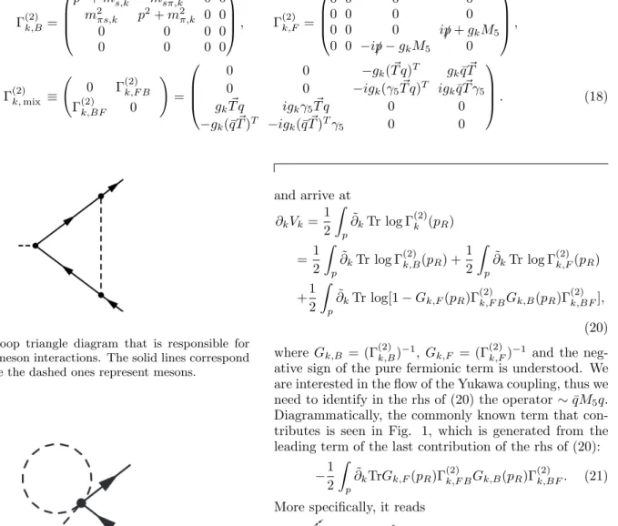
FIG. 1. One loop triangle diagram that is responsible for flowing quark–meson interactions. The solid lines correspond to quarks, while the dashed ones represent mesons.

FIG. 2. One loop tadpole diagram arising from the field de- pendent Yukawa interaction, which allows the generation of new quark–meson vertices in the RG flow. The solid lines cor- respond to quarks, while the dashed ones represent mesons.

Using these notations, and by introducing the differential operator ˜∂k, which, by definition acts only on the regula- tor function,R_k, (14) can be conveniently reformulated.

We may use the matrix identity

Γ⁽²⁾_k,B Γ⁽²⁾_k,BF Γ⁽²⁾_{k,F B} Γ⁽²⁾_k,F

!

= Γ⁽²⁾_k,B 0 Γ⁽²⁾_{k,F B} 1

! 1 (Γ⁽²⁾_k,B)⁻¹Γ⁽²⁾_k,BF 0 Γ⁽²⁾_k,F −Γ⁽²⁾_{k,F B}(Γ⁽²⁾_k,B)⁻¹Γ⁽²⁾_k,BF

!

(19)

and arrive at

∂kVk =1 2

Z

p

∂˜kTr log Γ⁽²⁾_k (pR)

= 1 2 Z

p

∂˜kTr log Γ⁽²⁾_k,B(pR) +1 2 Z

p

∂˜kTr log Γ⁽²⁾_k,F(pR) +1

2 Z

p

∂˜kTr log[1−Gk,F(pR)Γ⁽²⁾_{k,F B}Gk,B(pR)Γ⁽²⁾_k,BF], (20) where G_k,B = (Γ⁽²⁾_k,B)⁻¹, G_k,F = (Γ⁽²⁾_k,F)⁻¹ and the neg- ative sign of the pure fermionic term is understood. We are interested in the flow of the Yukawa coupling, thus we need to identify in the rhs of (20) the operator∼qM¯ 5q.

Diagrammatically, the commonly known term that con- tributes is seen in Fig. 1, which is generated from the leading term of the last contribution of the rhs of (20):

−1 2

Z

p

∂˜kTrGk,F(pR)Γ⁽²⁾_{k,F B}Gk,B(pR)Γ⁽²⁾_k,BF. (21) More specifically, it reads

× G^ab_k,s(p_R)−G^ab_k,π(p_R) +iγ₅[G^ab_k,sπ(p_R) +G^ab_k,πs(p_R)]

T_bo q,(22) whereS_k(p) = (i/p+g_kM₅)⁻¹ is the fermion propagator without doubling, while G_k,s, G_k,π, and G_k,sπ are the respective 9×9 submatrices ofGk,B in a purely bosonic background (see Appendix B). In principle, the evalua- tion of (22) goes as follows. First, one evaluates Γk,B, then inverts it to obtain G_k,s, G_k,π and G_k,sπ. Sec- ond, one inverts the fermion propagator, and finally per- forms all matrix multiplications to get the operator that is sandwiched by ¯qandq. Note that the procedure turns out to be too complicated to be carried out in a general background, but as we explain in the next subsections, fortunately we will not need to evaluate (22) in its full generality.

On top of the above, via a field dependent Yukawa coupling there is also contribution from the first term of (20), as meson masses get modified by a fermionic background (see Appendix B) leading to the possiblity of generating a∼qM¯ ₅q term in the effective action, see Fig. 2. Generically this contributes to the rhs of (20) as

= ¯qg⁰_k(ρ) 2

Z

p

∂˜k

n

G^ab_k,s(pR)∂ρ

∂sa

∂M5

∂sb

+ ∂ρ

∂sb

∂M5

∂sa

+δabM5

+G^ab_k,π(pR) ∂ρ

∂πa

∂M5

∂πb

+ ∂ρ

∂πb

∂M5

∂πa

+δabM5

,

+G^ab_k,sπ(pR) ∂ρ

∂πb

∂M5

∂sa

+ ∂ρ

∂sa

∂M5

∂πb

+G^ab_k,πs(pR) ∂ρ

∂πa

∂M5

∂sb

+ ∂ρ

∂sb

∂M5

∂πa

o q

+¯qg_k⁰⁰(ρ) 2

Z

p

∂˜k

n

G^ab_k,s(pR)∂ρ

∂sa

∂ρ

∂sb

+G^ab_k,π(pR)∂ρ

∂πa

∂ρ

∂πb

+G^ab_k,sπ(pR)∂ρ

∂sa

∂ρ

∂πb

+G^ab_k,πs(pR)∂ρ

∂sb

∂ρ

∂πa

o

M5q. (23)

A. Flows in the symmetric phase

As a first step, we are interested in the RG flows in the symmetric phase, i.e., where they are obtained at zero field. Note that, however, this still necessitates the eval- uation of the rhs of the flow equation (22) in a nonzero background, but if we are interested in the flowing cou- plings of dimension 6 operators, it is sufficient to perform all computations at the cubic order in the meson fields.

That is to say, when all propagators are expanded around M = 0 (see Appendix B for the general formulas), one is allowed to work with them at the following accuracy:

G^ab_k,s(p) = 1

p²+U_k⁰δ_ab− 1 (p²+U_k⁰)²

×

s_as_bU_k⁰⁰+ ∂²τ

∂sa∂sb

C_k

, (24a)

G^ab_k,π(p) = 1

p²+U_k⁰δab− 1 (p²+U_k⁰)²

×

πaπbU_k⁰⁰+ ∂²τ

∂πa∂πb

Ck

, (24b)

G^ab_k,sπ(p) =− 1 (p²+U_k⁰)²

s_aπ_bU_k⁰⁰+ ∂²τ

∂sa∂πb

C_k , (24c) Sk(p) =−i/p

p² +g_kM₅^†

p² , (24d)

where the coefficient functions (i.e. U_k⁰, U_k⁰⁰, Ck) are evalu- ated at zero field. Note that in this subsection all compu- tations are performed without specifying any background field and keeping its most general form. Terms that con- tain higher derivatives ofC_kare left out since their coeffi- cients would lead to subleading (higher than cubic power) contributions in the background fields in (22) and (23).

Note that the scalar and pseudoscalar meson propaga- tors do not mix in the symmetric phase and are degener- ate, therefore, there is a relative (−1) factor between their contributions in (22), which exactly cancels the term lin- ear in the mesonic fields. In the piece of the integrand that is quadratic in them the quark momentum is odd, therefore, upon integration it also vanishes. The leading

contribution of (22) is determined by the mass terms:

×h

(sasb−πaπb)U_k⁰⁰+ ∂²τ

∂sa∂sb

Ck− ∂²τ

∂πa∂πb

Ck

+iγ₅(s_aπ_b+s_bπ_a)U_k⁰⁰+iγ₅C_k ∂²τ

∂sa∂πb

+ ∂²τ

∂πa∂sb

iT_bq.

(25) Exploiting various identities of theU(3) algebra (see Ap- pendix A), one can perform the algebraic evaluation of the integrands to arrive at:

×h

g_k³U_k⁰⁰−2 3g³_kC_k

¯

q M₅M₅^†−ρ/3 M₅q + 1

3g³_kU_k⁰⁰+16 9 g_k³Ck

ρ¯qM5qi

. (26) Eq. (26) clearly shows the appearance of a new dimen- sion 6 operator (∼qM¯ ₅M₅^†M₅q), which was absent in the ansatz of the effective action. Before discussing this re- sult, let us turn to the contribution of (23). Using, again, expressions (24), a straightforward calculation leads to

= Z

p

∂˜_k 1 p²_R+U_k⁰

h10g_k⁰qM¯ ₅q+g⁰⁰_kρ¯qM₅qi +

Z

p

∂˜_k 1 (p²_R+U_k⁰)²

h(−16

3 g⁰_kC_k−3g⁰_kU_k⁰⁰)ρ¯qM₅q

−6g⁰_kCkq M¯ 5M₅^†−ρ/3 M5qi

,(27) where the coefficient functions (i.e. U_k⁰, g_k, g_k⁰, g_k⁰⁰, C_k) are, once again, evaluated at zero field. The flow of the effec- tive potential is the sum of (26) and (27).

At this point it is clear that the flow equation does not close in the sense that the ansatz (15) does not contain the operator ∼ qM¯ 5M₅^†M5q, therefore, for consistency reasons, it has to be dropped also in the rhs of (20).

Instead of doing so, one may choose to project out the

∼q(M¯ 5M₅^† −ρ/3)M5q term, because in the symmetry breaking pattern UL(3)×UR(3) → UV(3) that is the actual combination, which vanishes. This choice should lead to the appropriate definition of the field dependent flowing Yukawa coupling if no explicit symmetry breaking

terms are present. Note, however, that, once finite quark masses and the corresponding explicit breaking terms are introduced, in the minimum point of the effective poten- tialM5M₅^†6=ρ/3, and the aforementioned projection can be regarded as somewhat arbitrary. A more appropriate treatment is to include ∼qM¯ 5M₅^†M5q in the ansatz of the effective action in the first place (see Sec. IV).

We close this subsection by listing the coupled flow equations for the Yukawa coupling and its derivative eval- uated at zero field, i.e. in the symmetric phase, when

∼q(M¯ ₅M₅^†−ρ/3)M₅q is projected out. Dropping g⁰⁰_k in order to close the system of equations, and by using the definitions of (9), (26) and (27) we are led to

∂kg0,k= 10g1,k

Z

p

∂˜k

1

p²_R+U_k⁰, (28a)

∂kg1,k=1

3g_0,k³ U_k⁰⁰+16 9 g_0,k³ Ck

Z

p

∂˜k

1 p²_R(p²_R+U_k⁰)²

−16

3 g1,kCk+ 3g1,kU_k⁰⁰Z

p

∂˜k

1

(p²_R+U_k⁰)².(28b)

B. Flows in the broken phase

Now we explore how the flowing couplings depend on the fields, more specifically, as described in (8), their ρ dependence will be determined.

At this point, we specify a background in which we will evaluate the flow equation, as in case of general{M,

¯

q, q} configurations, there is no hope that the broken symmetry phase calculations can be done explicitly. The nice thing, however, is that it is sufficient to work in a restricted background. We, again, definitely need to assume nonzero ¯q,q, and then we specify theM =s0T0+ s8T8 “physical” condensate. This is one of the minimal choices, which allows for a unique restoration of the ∼

¯

qM5M₅^†M5qand∼qM¯ 5qoperators in the rhs of the flow equation (a one component condensate would definitely not allow to do so). We have checked explicitly with other backgrounds the uniqueness of the results, and as

expected, found agreement.

As outlined above, the first step is to evaluate the 2–

point functions Γ⁽²⁾_k,s, Γ⁽²⁾_k,π (note that in the current back- ground there is nos−πmixing), see details in Appendix B, in particular (B10) and (B11). Then one inverts these matrices to obtainGk,sandGk,π. They are diagonal ex- cept for the 0–8 sectors. Similarly, for the fermion prop- agator, one hasS_k⁻¹(p) = (i/p+gk(ρ)M5), which leads to the inverse

Sk(p) = −i/p+gkM₅^†

p²+gkM5M₅^†. (29) Since in the background in question [Sk, M5] = 0, Eq.

(22) becomes

× Z

p

∂˜_kn

T_aS_k²(p_R)M₅ G^ab_k,s(p_R)−G^ab_k,π(p_R) T_bo

q.

(30) Similarly, exploiting the choice of the simplified back- ground, (23) becomes

= ¯qg_k⁰⁰(ρ) 2

Z

p

∂˜kG^ab_k,s(pR)sasbq + ¯qg_k⁰(ρ)

2 Z

p

∂˜k

G^ab_k,s(pR)(saTb+sbTa) +(G^aa_k,s(pR) +G^aa_k,π(pR))M5

q.(31) It is important to mention that one does not need to work with generals0,s8background values, but can safely as- sume thats8s0, and thus expand both (30) and (31) in terms ofs8and work in the leading order. This simpli- fication still uniquely allows for identifying the flow of the

∼qM¯ 5q and ∼q(M¯ 5M₅^†−ρ/3)M5q operators. The lat- ter, as expected, pops up again [it is inherently ofO(s₈)], thus a two component background is indeed necessary to obtain each flow. The sum of (30) and (31) leads to

Z

p

∂˜k

3 2g⁰_k(ρ)

3

p²_R+U_k⁰(ρ)+ 8

3p²_R+ 4Ck(ρ)ρ+ 3U_k⁰(ρ)+ 1

p²_R+U_k⁰(ρ) + 2ρU_k⁰⁰(ρ)

¯ qM5q,

+ Z

p

∂˜_k

g³_k(ρ)(3p²_R−g_k²(ρ)ρ)

16Ck(ρ)(p²_R+U_k⁰) + 3 p²_R+ 12Ck(ρ)ρ+U_k⁰(ρ) U_k⁰⁰(ρ) (3p²_R+g_k²(ρ)ρ²

p²_R+U_k⁰(ρ)

3p²_R+ 4C_k(ρ)ρ+ 3U_k⁰(ρ)

p²_R+U_k⁰(p_R) + 2ρU_k⁰⁰(ρ) + g⁰⁰_k(ρ)

p²_R+U_k⁰(ρ) + 2ρU_k⁰⁰(ρ)

! ρ¯qM5q,

+ Z

p

∂˜_k 2g_k³(ρ)(3p²_R−g²_k(ρ)ρ) A₀+A₁(p²_R+U_k⁰(ρ)) +A₂(p²_R+U_k⁰(ρ))² 6p²_R+ 2g_k²(ρ)ρ3

p²_R+U_k⁰(ρ)2

3p²_R+ 4Ck(ρ)ρ+ 3U_k⁰(ρ)2

p²_R+U_k⁰(ρ) + 2ρU_k⁰⁰(ρ)

− 6g_k⁰(ρ)(3Ck(ρ) + 2C_k⁰(ρ)ρ) 3p²_R+ 4Ck(ρ)ρ+ 3U_k⁰(ρ)

p²_R+U_k⁰(ρ) + 2ρU_k⁰⁰(ρ)

!

¯

q(M5M₅^†−ρ/3)M5q, (32)

where

A₀=−288C_k³(ρ)ρ² 3p²_R+g²_k(ρ)ρ

k²+U_k⁰(ρ) + 2ρU_k⁰⁰(ρ)

+ 36(p²_R+U_k⁰(ρ))³ 4C_k(ρ)ρ(3p²_R+g_k²(ρ)ρ) + 9p²_RU_k⁰⁰(ρ) , A1=−144C_k²(ρ)ρ

14p²_R+ 4g²_k(ρ)ρ

p²_R+U_k⁰(ρ)

+ 12ρU_k⁰⁰ 3p²_R+g²_k(ρ)ρ , A2=−12Ck(ρ)

18p⁴_R+ 6p²_R 3U_k⁰(ρ) + 12ρU_k⁰⁰(ρ)−8C_k⁰(ρ)ρ²

+ 4g²_k(ρ)ρ² 9U_k⁰⁰(ρ)−4Ck(ρ)ρ .

As in the previous subsection, we may drop the last term in (32) due to consistency and thus the first two terms provide the result for the fully non-perturbative flow of the Yukawa coupling. One can check explicitly that ex- panding (32) around ρ= 0 leads back to the earlier re- sults of (27).

The expression obtained for the flow of the Yukawa coupling gk(ρ) is thought to be a resummation of oper- ators as described below (9). As such, one is able to determine how strong the interaction is between quarks and mesons as e.g. the chiral condensate evaporates at high temperature. In principle g_k(ρ) also depends ex- plicitly on the temperature but one expects that the de- crease in ρ is more important [5]. For phenomenology, e.g. parametrization, or mass spectrum calculation, one needs to evaluate gk(ρ) and its derivatives at the mini- mum point of the effective potential,ρ=ρ_min.

IV. EFFECT OF THEM5M₅^†M5 OPERATOR

Motivated by the nonuniqueness of the definition of the field dependent Yukawa coupling in the earlier setting, now we investigate the case when the term R

xg_53,kqM¯ ₅M₅^†M₅q is added to the ansatz (15) of the effective action (without substractingρ¯qM₅q/3 from it).

Here g53,k is a new running coupling constant, and we will not be considering its field dependence. Also, we re- strict ourselves to calculations in the symmetric phase, therefore, a similar treatment as of in Sec. IIIA is in or- der. All calculations presented there are still valid, but there is one more term contributing to rhs of the flow equation of the effective action, coming from the tadpole diagram of Fig. 2 [see the mass matrices in (B9)]:

¯ qg₅₃

2 Z

p

∂˜_k[G^ij_k,s(p_R)

M₅,{Ti, T_j} +T_iM₅^†T_j+T_jM₅^†T_i +G^ij_k,π(pR)(

M5,{Ti, Tj} −TiM₅^†Tj−TjM₅^†Ti) +G^ij_k,sπ(pR)iγ5(

M5,[Ti, Tj]

+TiM₅^†Tj+TjM₅^†Ti) +G^ij_k,πs(p_R)iγ₅(

M₅,[T_j, T_i]

+T_iM₅^†T_j+T_jM₅^†T_i)]q.

(33) Substituting the propagators from Eqs. (24), without specifying an actual background field, straightforward

calculations lead to 6g53,kqM¯ 5q

Z

p

∂˜k

1 p²_R+U_k⁰ −

2g53,kCkρ¯qM5q +(3g53,kU_k⁰⁰+ 10g53,kCk

qM¯ 5M₅^†M5q Z

p

∂˜k

1 (p²_R+U_k⁰)².

(34) Note that all couplings (i.e. U_k⁰, U_k⁰⁰, Ck) are evaluated at zero field as we have worked in the symmetric phase.

One observes that even though the original (field inde- pendent) Yukawa coupling does not flow in the symmet- ric phase, once one includes theg₅₃ coupling, it does run with respect to the scale. Using (28a), (28b) and (34), we arrive at the following system of equations for g0,k, g1,k andg53,k:

∂_kg_0,k= (10g_1,k+ 6g_53,k) Z

p

∂˜_k 1

p²_R+U_k⁰, (35)

∂kg1,k=−10

3 g1,kCk+ 3g1,kU_k⁰⁰+ 2g53,kCk

× Z

p

∂˜k

1

(p²_R+U_k⁰)² + 2g³_0,kCk

Z

p

∂˜k

1 p²_R(p²_R+U_k⁰)²,

(36)

∂kg53,k=−(6g1,kCk+ 10g53,kCk+ 3g53,kU_k⁰⁰)

× Z

p

∂˜_k 1

(p²_R+U_k⁰)² + (g_0,k³ U_k⁰⁰−2 3g³_0,kC_k)

× Z

p

∂˜_k 1

p²_R(p²_R+U_k⁰)². (37) We wish to note that based on Sec. IIIB, a broken phase calculation can also be done. This, however, leads to such complicated formulas that we do not go into the details.

V. SUMMARY

In this paper we raised the question of determining the field dependence of the Yukawa coupling in the three fla- vor quark–meson model. Our main motivation was to clarify the problem of consistency between chiral sym- metry and the Yukawa term. As opposed to two flavors, in case of three flavors, the existence of non Yukawa–like interactions and their generation in the infrared scales of the quantum effective action prevents a straightforward generalization of the two flavor approach [10]. That is to say, one cannot consistently work with e.g. a scalar

chiral condensate and associate the complete field depen- dence of the quark–quark–meson vertex with that of the Yukawa coupling itself. One needs great care to project out those operators that are not included in the ansatz of the effective action, which, by construction, need to re- spect chiral symmetry. We believe that such a consistent approach was missing in the literature so far.

We have explicitly calculated the renormalization group flow of the field dependent Yukawa coupling sep- arately in the symmetric and broken phases. We have showed that at the order of dimension 6 operators new type of terms arise, and argued how to project them out required by consistency. Motivated by the very definition of the flow of the field dependent Yukawa coupling, for the sake of a complete treatment of dimension 6 opera- tors, we have determined the symmetric phase flows when these new (non-renormalizable) interactions are also em- bedded into the ansatz of the quantum effective action (Γk).

It would be very important to see what effects the cur- rent approach has from a phenomenological point of view.

One is typically interested in mapping the details of the chiral phase transition at finite temperature and/or den- sity, such as the transition point, mass spectrum, interac- tion strengths, etc. To do so one also needs to include t’

Hooft’s determinant term into the system describing the UA(1) breaking, and it would be of particular interest to check the interplay between the anomaly coupling and that of the Yukawa interaction. These directions repre- sent future studies to be reported elsewhere.

ACKNOWLEDGEMENTS

The authors thank Zs. Sz´ep for useful discussions re- lated to the perturbative renormalization of the Yukawa coupling. This research was supported by the Hungarian National Research, Development and Innovation Fund under Project Nos. PD127982 and K104292. G.F. was also supported by the J´anos Bolyai Research Scholar- ship of the Hungarian Academy of Sciences, and by the UNKP-20-5 New National Excellence Program of the´ Ministry for Innovation and Technology from the source of the National Research, Development and Innovation Fund.

Appendix A. U(3) ALGEBRA IDENTITIES

TheU(3) algebra is spanned by the 3×3T_i(i= 0, ...8) generators, which satisfy Tr (T_iT_j) =δ_ij/2, and a prod- uct of two generators lie in the Lie algebra:

T_iT_j =1

2(d_ijk+if_ijk)T_k. (A1)

Associativity of matrix multiplication leads to the follow- ing identities:

0 =f_ilmf_mjk+f_jlmf_imk+f_klmf_ijm, (A2a) 0 =filmdmjk+fjlmdimk+fklmdijm, (A2b) 0 =fijmfklm−dikmdjlm+djlmdilm, (A2c) the first one known as the Jacobi identity. Using that T_iT_i is a Casimir operator, working in the adjoint repre- sentation one easily shows thatfijkfljk= 3δil(1−δi0δl0).

Using this identity as a starting point, one derives the fol- lowing 2 and 3-fold sums using (A2):

dijmdkjm= 3δik+ 3δi0δk0, (A3a) flnifikmfmjl=−3

2fnkj, (A3b)

dmikdknjfjlm= 3

2finl, (A3c)

finlfljmdmki= r3

2(δn0δjk+δj0δnk−δk0δnj),

−3

2dnjk (A3d)

dikldlnmdmji= r3

2(δn0δjk+δj0δnk+δk0δnj) +3

2d_njk. (A3e)

Furthermore, the following identities for 4-fold sums are useful for present calculations:

diajdjbkdkcldldi=3

4(dabmdmcd+dadmdmcb)−3

4dacmdmbd

+1

2(δabδcd+δacδbd+δadδbc) +1

2 r3

2(δa0dbcd+δb0dacd+δc0dabd+δd0dabc), (A4a) f_iajd_jbkd_kcld_ldi+f_iajd_jbkd_kdld_lci =f_abjd_ijkd_kcld_ldi,

(A4b) fiajdjckdkdldlbi+fiajdjdkdkcldlbi =fabjdijkdkcldldi

+2f_bdjf_lakf_kjmd_mcl+ 2f_bcjf_ljkf_kamd_mdl. (A4c)

Appendix B. INVARIANT TENSORS AND TWO POINT FUNCTIONS

First we recall that

ρ= Tr (M^†M), (B1a)

τ= Tr (M^†M− Tr (M^†M)/3)², (B1b)

whereM = (s_i+iπ_i)T_i. In terms ofs_iandπ_i, they read ρ= 1

2(s_is_i+π_iπ_i), (B2a) τ= 1

24(s_is_js_ks_l+π_iπ_jπ_kπ_l)D_ijkl +s_is_jπ_kπ_l( ˜D_ij,kl−D_ijkl/4)

− 1

12(s_is_i+π_iπ_i)², (B2b) where D_ijkl = d_ijmd_klm + d_ikmd_jlm + d_ilmd_jkm and D˜ij,kl = dijmdklm. The relevant derivatives of ρ and τ are

∂ρ

∂s_i =si, ∂ρ

∂π_i =πi, (B3a)

∂²ρ

∂sisj

=δij, ∂²ρ

∂πiπj

=δij, (B3b)

∂τ

∂s_i =−2 3ρsi+1

6sasbscDabci

+1

2s_aπ_cπ_d(4 ˜D_ai,cd−D_aicd), (B4a)

∂τ

∂π_i =−2 3ρπi+1

6πaπbπcDabci

+1

2π_as_cs_d(4 ˜D_ai,cd−D_aicd), (B4b)

∂²τ

∂si∂sj

=−2

3ρδij−2

3sisj+1

2sasbDabij

+1

2πcπd(4 ˜Dij,cd−Dijcd), (B4c)

∂²τ

∂πi∂πj

=−2

3ρδ_ij−2

3π_iπ_j+1

2π_aπ_bD_abij +1

2scsd(4 ˜Dij,cd−Dijcd), (B4d)

∂²τ

∂π_i∂s_j =−2

3π_is_j+s_aπ_c(4 ˜D_aj,ci−D_ajci). (B4e)

In case of the broken phase calculation, we are working in a background fieldM =s0T0+s8T8, thus the following formulas need to be used. First we list the invariants:

ρ|s₀,s₈= 1

2(s²₀+s²₈), (B5a) τ|s₀,s₈= 1

24s²₈(8s²₀−4√

2s0s8+s²₈). (B5b)

Then, the nonzero first derivatives are

∂ρ

∂s0

_s

0,s₈

=s₀, ∂ρ

∂s8

_s

0,s₈

=s₈, (B6a)

∂τ

∂s_{0 s}

0,s₈

=s²₈2s0

3 − s8

3√ 2

, (B6b)

∂τ

∂s_{8 s}

0,s₈

=s8

2s²₀ 3 −s0s8

√2 +s²₈ 6

. (B6c)

As shown above, the second derivatives ofρare equal to the unit matrix, while that ofτ are the following:

∂²τ

∂sisj

_s

0,s₈

=























2

3s²₈, if i=j= 0

−^√s28₂+⁴₃s₀s₈, if i= 0, j= 8 or i= 8, j= 0

2

3s²₀+^s₂²⁸ −√

2s₀s₈, if i=j = 8

2

3s²₀+^s₆²⁸ +√

2s0s8, if i=j = 1,2,3

2

3s²₀+^s₆²⁸ −^√1

2s0s8, if i=j= 4,5,6,7

0, else

(B7a)

∂²τ

∂πiπj

_s

0,s8

=























0, if i=j= 0

− ^s28

3√

2+²₃s0s8, if i= 0, j= 8 or i= 8, j= 0

s²₈ 6 −

√2

3 s0s8, if i=j = 8

−^s₆²⁸ +

√2

3 s₀s₈, if i=j= 1,2,3

5 6s²₈− ¹

3√

2s0s8 if i=j= 4,5,6,7

0, else

. (B7b)