How well can screening sensitivity and sojourn time be estimated ∗

(1)

How well can screening sensitivity and sojourn time be estimated ^∗

Ayman Hijazy

^ab

, András Zempléni

^a

aDepartment of Probability Theory and Statistics, Eötvös Loránd University aymanhijazy@caesar.elte.hu

bFaculty of Informatics, University of Debrecen andras.zempleni@ttk.elte.hu

Submitted: December 22, 2020 Accepted: March 8, 2021 Published online: May 18, 2021

Abstract

Chronic disease progression models are governed by two main parameters:

preclinical intensity and sojourn time. The estimation of these parameters helps in optimizing screening programs (with an additional parameter: sensitivity of the screens), and we examine their effect in improving survival.

Multiple approaches exist for estimating these parameters. However, these models are based on strong underlying assumptions. Our main aim is to investigate the effect of these assumptions. For this purpose, we developed a simulator to mimic a breast cancer screening program while directly observing the exact onset and the sojourn time of the disease. We then examine the performance of the model under different parameterizations and investigate the effects of different models on the sensitivity, the inter-screening intervals and misspecification of the used parametric distributions. Our results indicate a strong correlation among the estimated parameters. Besides, the underlying assumptions have a strong effect on the overall performance of the model.

These findings shed a light on the seemingly discrepant results obtained by different authors using the same data sets but different assumptions.

Keywords:Disease progression, likelihood, screening sensitivity, sojourn time

∗The project has been supported by the European Union, co-financed by the European Social Fund (EFOP-3.6.2-16-2017-00015).

doi: https://doi.org/10.33039/ami.2021.03.001 url: https://ami.uni-eszterhazy.hu

139

(2)

1. Introduction

Statistical modeling of natural disease progression aids in understanding its dynam- ics and forecasting its incidence rates. This allows better prevention and treatment plans which improves survival. However, in many cases, some data is not observ- able, as some diseases have an asymptomatic phase in which the patient does not know he has the sickness yet.

In the model proposed by Shen and Zelen [12], the natural progression of a disease is regarded as a three state model (see Figure 1): individuals progress from a disease free state 𝑆𝑓 to the preclinical state 𝑆𝑝, when the disease has become onset but is still asymptomatic, i.e. the person has the disease but it has not shown any symptoms. The final state of the disease from this point of view is when it manifests itself through clinical symptoms, thus it is called the clinical state𝑆𝑐.

𝑆𝑓 𝑆𝑝 𝑆𝑐

Figure 1. Progression in the three state model.

The flow in the process is governed by the preclinical intensity and the sojourn time. The preclinical intensity is the probability of moving from the disease free state to the preclinical one during(𝑡, 𝑡+𝑑𝑡). Equivalently, it is the waiting time in the disease free state 𝑆𝑝. The sojourn time is defined as the amount of time spent in the preclinical state𝑆𝑝, in other words it is the time needed for the disease to show itself by means of clinical symptoms. However, directly observing sojourn time is not feasible as the exact time of onset is unknown. The sojourn time is then estimated through modelling, mostly by assuming it is a random variable with a specified distribution, see e.g. [16, 17].

Early detection methods such as screening allows discovering the disease before any symptoms appear. Screening sensitivity, defined as the probability of detection given that the patient is in𝑆𝑝, is crucial in determining the efficiency of the screening program.

The parameters of interest in such a process are the preclinical intensity, the sojourn time and screening sensitivity. The estimation of these parameters is es- sential to optimize screening intervals and to correct lead time bias, that is defined as the apparent increase in survival due to early detection by means of screening.

In this paper we aim to investigate the identifiability of the parameters governing the process in different setups. For that purpose, a simulator is developed to record the exact onset and sojourn times of patients. This allows us to assess the accuracy of the estimators by comparing the estimated values to the real ones.

The theoretical basis of disease progression models under periodic screening was set by Zelen and Feinleib [17] and Prorok [10]. Later, Shen and Zelen [12] intro-

(3)

duced two models to estimate the parameters governing disease progression. The first describes stable diseases that are assumed to have incidence and prevalence independent of time or age. The other incorporates time dependence of incidence and prevalence to the model (these cases are called non stable diseases). We investigate the common cases, when incidence is age-dependent.

Wu et al. [16] further extended the results by allowing both the transition probability from the disease-free state and the sensitivity to be age-dependent.

They assume that the sojourn time follows a loglogistic distribution, the preclinical intensity has a lognormal distribution and the sensitivity is age-dependent, the age- dependence is incorporated by assuming that the sensitivity has a logistic function form.

Generally, these models are built by deriving the probabilities of cases being detected by screening or symptoms, this allows the forming a likelihood function from which parameters can be estimated by classical methods such as maximization of the likelihood function, a least squares approach or a Bayesian one. However, many questions can be raised about the effects of the assumptions one makes when modelling such a scenario.

The paper is organized as follows: we lay the model foundations in Section 2. Next, we setup the simulations in Section 3, we then present our simulation based on results in Section 4. We then show the reasons behind the discrepancy of estimates in the literature in Section 5. Finally, we summarize our findings in Section 6.

2. The model

We will use the generalized model proposed by Wu et al. [16] in this paper. Now, to lay the setup of the model, we suppose an individual becomes onset at a random time 𝑋 where 𝑋 is a random variable with a (possibly) defective density 𝑓𝑋(𝑥).

Introduce 𝑟 ≤ 1 as the lifetime risk, which is the probability of a person to get the disease i.e. ∫︀∞

0 𝑓𝑋(𝑥) d𝑥=𝑟. After a case becomes onset, we suppose that it stays in the preclinical state for a random amount of time𝑌 (called sojourn time) independent of 𝑋, where 𝑌 is a random variable with pdf 𝑓𝑌(𝑦) and survivor function 𝑄𝑌(𝑦). Let 𝑍 =𝑋+𝑌 denote the time of diagnosis. As 𝑋 and 𝑌 are assumed independent, the density of𝑍 in the absence of screening is given by the convolution of𝑋 and𝑌, namely: 𝑓𝑍(𝑧) =∫︀𝑧

0 𝑓𝑋(𝑥)𝑓𝑌(𝑧−𝑥) d𝑥.

If no screens are organized, i.e. the patient only knows that he has the sickness when symptoms are exhibited, then one can only observe the time of diagnosis𝑍 and the likelihood function would simply be the product of the densities 𝑓𝑍(𝑧𝑖).

The identifiablity of the parameters in such a setup is a serious concern, for instance if both 𝑋 and 𝑌 are normally distributed, there are infinitely many parameters which can generate the same distributions. We currently investigate the theoretical aspects of identifiability which we will publish in a separate paper.

Suppose now that a screening program consisting of𝐾screens is organized for a population which is stratified by age at the first screen𝑡1where𝑡1=𝑡_min, . . . , 𝑡_max.

(4)

Let us define ∆ as the inter-screening time and assume that all participants are disease free at age 𝑡0 before the first screen (we assume𝑡0 = 0). Denote by𝑡𝑖 = 𝑡1+ (𝑖−1)∆the age at the𝑖^𝑡ℎ screen and by(𝑡_𝑖−1, 𝑡𝑖)the𝑖^𝑡ℎ screening interval.

Denote the sensitivity of a screen by𝜉(𝑡)and suppose it is a parametric function of the age at screening. The aim is to build a likelihood function using the probabilities of detection by screens and by showing symptoms.

Under this setup, the probability of detection at the first screen for those aged 𝑡1at the first screen denoted by𝐷1,𝑡1 is given by cases which have moved to𝑆𝑝in (𝑡0, 𝑡1)and stayed there till they are screened positively. Therefore:

𝐷1,𝑡1 =𝜉(𝑡1)

𝑡1

∫︁

𝑡0

𝑓𝑋(𝑥)𝑄𝑌(𝑡1−𝑥) d𝑥.

In order to determine the probability of detection at the 𝑘^𝑡ℎ screen, let us discretize the timeline into intervals of the form (𝑡_𝑖−1, 𝑡𝑖). Denote by 𝐷^(𝑖)_𝑘,𝑡₁ the contribution of cases which have moved to 𝑆𝑝 in the𝑖^𝑡ℎ screening interval to the probability of detection at the𝑘^𝑡ℎ screen for𝑖= 1, . . . , 𝐾. That is given by cases which have been falsely screened negative in all the previous screens and they did not show symptoms before the𝑘^𝑡ℎscreen when they were finally screened positively.

Hence:

𝐷^(𝑖)_𝑘,𝑡₁=

⎧⎨

⎩ 𝜉(𝑡𝑘)[︁

(1−𝜉(𝑡𝑖))· · ·(1−𝜉(𝑡_𝑘−1))]︁∫︀𝑡𝑖

𝑡𝑖−1𝑓𝑋(𝑥)𝑄𝑌(𝑡𝑘−𝑥) d𝑥,if𝑖 < 𝑘, 𝜉(𝑡𝑘)∫︀𝑡𝑘

𝑡𝑘−1𝑓𝑋(𝑥)𝑄𝑌(𝑡𝑘−𝑥) d𝑥, if𝑖=𝑘.(2.1) Hence, the probability of detection at the 𝑘^𝑡ℎ screen is given by the sum of contributions:

𝐷𝑘,𝑡1=

∑︁𝑘 𝑖=1

𝐷^(𝑖)_𝑘,𝑡₁.

A similar approach is used to determine the probability of showing symptoms in the𝑘^𝑡ℎscreening interval. Denote by𝑓_𝑍^(𝑖,𝑘)_𝑡

1 the contribution of cases which have moved to𝑆𝑝in(𝑡𝑖−1, 𝑡𝑖)to the probability of showing symptoms between(𝑧, 𝑧+𝑑𝑧) where𝑡_𝑘−1< 𝑧 < 𝑡𝑘. Therefore:

𝑓_𝑍^(𝑖,𝑘)_𝑡

1 (𝑧) =

⎧⎨

⎩

∫︀𝑧

𝑡𝑘−1𝑓𝑋(𝑥)𝑓𝑌(𝑧−𝑥) d𝑥, if𝑘=𝑖,

∫︀𝑡𝑖

𝑡𝑖−1𝑓𝑋(𝑥)𝑓𝑌(𝑧−𝑥) d𝑥∏︀𝑘−1

𝑗=𝑖(1−𝜉(𝑡𝑗)), if𝑘 > 𝑖. (2.2) Hence, the probability of a case to show symptoms between𝑧 and 𝑧+𝑑𝑧 for 𝑡𝑘< 𝑧 < 𝑡𝑘+1is given by:

𝑓_𝑍^𝑘_𝑡

1(𝑧) =

∑︁𝑘 𝑖=1

𝑓_𝑍^(𝑖,𝑘)_𝑡

1 (𝑧). (2.3)

(5)

The probability for a case to show symptoms between𝑡𝑘−1and𝑡𝑘for individuals aged𝑡1 at the first screen denoted by𝐼𝑘,𝑡1 is given by integrating Equation (2.3), i.e.

𝐼𝑘,𝑡1 =

𝑡𝑘

∫︁

𝑡𝑘−1

𝑓_𝑍^𝑘_𝑡

1(𝑧) d𝑧.

For a screening program consisting of𝐾screens and participants age at first screen ranging between𝑡_min, . . . , 𝑡_max, Wu et al. [16] used the count data(𝑛𝑘,𝑡1, 𝑠𝑘,𝑡1, 𝑟𝑘,𝑡1) to form a likelihood function similar to a multinomial distribution, where 𝑛𝑘,𝑡1 is the number of participants in screen𝑘 who were aged𝑡1at program entry,𝑠𝑘,𝑡1 is the number of screen detected cases on screen𝑘from those aged𝑡1at screen entry and 𝑟𝑘,𝑡1 is the number of symptomatic cases in the 𝑘^𝑡ℎ screening interval from those aged𝑡1at program entry. The likelihood is of the form:

𝐿1=

𝑡∏︁_max

𝑡1=𝑡_min

∏︁𝐾 𝑘=1

𝐼_𝑘,𝑡^𝑟^𝑘,𝑡₁¹𝐷_𝑘,𝑡^𝑠^𝑘,𝑡₁¹(1−𝐷𝑘,𝑡1−𝐼𝑘,𝑡1)^𝑛^𝑘,𝑡¹⁻^𝑠^𝑘,𝑡¹⁻^𝑟^𝑘,𝑡¹.

Our important suggestion is that we propose to incorporate the exact dates of diagnosis of symptomatic patients (𝑧𝑖) in the likelihood function if they are available, as they carry important information. Then the likelihood is of the form:

𝐿2=

𝑡∏︁_max

𝑡1=𝑡_min

∏︁𝐾 𝑘=1

[︃

𝐷_𝑘,𝑡^𝑠^𝑘,𝑡₁¹(1−𝐷𝑘,𝑡1−𝐼𝑘,𝑡1)^𝑛^𝑘,𝑡¹⁻^𝑠^𝑘,𝑡¹⁻^𝑟^𝑘,𝑡¹

𝑟∏︁𝑘,𝑡1

𝑖=1

𝑓_𝑍^𝑘_𝑡

1(𝑧𝑖) ]︃

.

After specifying the parametric distributions of the preclinical and the sojourn time, we obtain the maximum likelihood estimates through nonlinear minimization of the negative log-likelihood. The variances of the parameter estimators can be approximated using the observed Fisher information matrix. We expect this to be more accurate for larger sample sizes.

3. Simulation setup

In order to investigate the identifiability of the parameters, we simulated disease progression data mimicking a breast cancer screening program using different onset and sojourn time distributions. The aims are: checking the identifiability of the parameters, examining the improvement in the model performance if the exact date of the diagnosis of symptomatic cases is incorporated, studying the effect of the length of the inter-screening time and see the effects of incorrect specifica- tions, namely if the sensitivity is falsely assumed constant or if the sojourn time distribution is misspecified.

Breast cancer’s screening sensitivity is known to be increasing with age ([11]).

Wu et al [16] choose to model this age-dependence via a logistic function with parameters 𝑏0 and𝑏1. As a result, the sensitivity at age𝑡is then given by:

𝜉(𝑡) = 1

exp(−𝑏0−𝑏1(𝑡−¯𝑡)).

(6)

Adopting the age-dependent sensitivity, we also chose the lognormal distribution 𝐿𝑁(𝜇, 𝑠²)for the onset time. This is realistic since the transition probabilities of breast cancer to the preclinical state were estimated by Lee and Zelen [8] using age- specific incidence rates. Wu et al [16] plotted the probabilities and found them to be right skewed with a heavy tail, so the lognormal distribution was chosen for having similar properties. It is also noted that the estimates of the onset distribution parameters may depend on the model choice, so different estimates exist [9]. We simulated our data using 𝜇= 3.971 and𝑠= 2.267, these values lead to an average age of transition of around 54 years and a standard deviation of 15 years.

Using a lognormal preclinical intensity and an age-dependent sensitivity, we simulate progression data based on an exponential sojourn time with 𝜆 = 1/2.5 and a gamma sojourn time with shape 𝛼= 6.25 and rate𝛽 = 2.5 both resulting in a mean sojourn time of 2.5 years and a unit variance (gamma case). For 𝑡1 = 40, . . . ,65 years, we simulate 2 data sets for each distribution, one with𝑁1,𝑡1 = 10 000 and the other of size 𝑁1,𝑡1 = 100 000in each cohort, this would help us study the asymptotic performance of the model. The model is then run on each of the data sets, with and without including the exact date of diagnosis.

We also run a simplified simulation mimicking the model used by Duffy et al [3] in which both the onset and the sojourn times are exponentially distributed with parameters 𝜆1 and 𝜆2 while assuming that the sensitivity is constant. From a mathematical point of view, this model is interesting as the natural progression (without screening) in the chain is time homogeneous. The defined parameters in the simulations are 𝜉 = 0.75, 𝜆1 = 1/55 and 𝜆2 = 1/2.5, resulting in an average onset age of 55 years and a mean sojourn time of 2.5 years. We also simulate two datasets (𝑁1,𝑡1 = 10 000and𝑁1,𝑡1 = 100 000).

In order to test the goodness of fit, we will use Pearson’s chi-squared test, which measures the distance between the observed and the expected counts. However, the chi-squared distance is just an illustrative measure, used only for showing the magnitude of the differences. Asymptotically, this distance is𝜒² distributed with 𝐾·(𝑡_max−𝑡_min)−𝑣 degrees of freedom, where𝑣is the number of parameters , but we experienced large deviations for the small sample sizes due to the large number of classes.

In order to establish confidence regions for the parameters, we will use the likelihood ratio statistic, which assesses the goodness of fit of two competing statistical models based on the ratio of their likelihoods. The likelihood ratio statistic can be expressed as a function of the difference between the loglikelihoods 𝐿𝑅= 2(𝑙(ˆ𝜃)−𝑙(𝜃)), where𝑙(ˆ𝜃)is the value of the loglikelihood at the maximum.

The finite sample distributions of likelihood-ratio tests are generally unknown.

However, under the null hypothesis (𝜃 = 𝜃0), 𝐿𝑅 converges in distribution to a 𝜒²-distribution (by Wilks’ theorem [15]). That allows defining the asymptotic confidence region𝐶(𝜃)as:

𝐶(𝜃) ={𝜃: 2(𝑙(ˆ𝜃)−𝑙(𝜃))< 𝜒²_0.95(𝑣)}.

The simulation and the nonlinear minimization of the negative loglikelihood are carried out using the statistical software R. However, since the integrals in

(7)

Equation (2.1) and (2.2) usually do not have a closed form, the integration has to be carried out numerically. This can be computationally expensive, especially as we include the date of diagnosis. For that reason, we use the packageRcpp [4] to carry out the numerical integration inC++using the packageCUBAby Hahn [5].

The negative of the log likelihood is then minimized using theoptim function, that is carried out using the “L-BFGS-B” algorithm [1]. In each scenario, we present the actual parameters, the estimates based on the count and full models for both data sets, the negative loglikelihood at the maximum (𝐿max) and the likelihood based on the actual parameters (𝐿𝑎𝑐𝑡𝑢𝑎𝑙).

4. Results

4.1. Exponential sojourn time

4.1.1. Exponentially distributed onset

Let us start with the results of the simplest case, in which a constant sensitivity is assumed along with exponential𝑋 and𝑌. The results are presented in Table 1, it is clear that the model does not perform well for a small sample size.

In the first block of Table 1, the results for the small data set are presented, we noticed that the estimates for both the count based and full model are similar but not accurate at all. The sensitivity and the average onset age are highly overestimated and the mean sojourn time is underestimated.

Table 1. Estimates of the sensitivity, onset and sojourn time parameters for exponentially distributed𝑋 and𝑌.

-Loglikelihood Sensitivity Onset Sojourn time

Maximum Actual 𝜉 1/𝜆1 1/𝜆2

Actual 0.75 55 2.5

∆ = 1 Count data 27 957.9 27 973.9 0.964 67.694 2.110 𝑁_𝑡₁= 10 000 Full data 27 950.4 27 975.9 1.000 59.443 2.081

∆ = 1 Count data 240 181.8 240 184.2 0.779 54.408 2.431 𝑁𝑡1= 100 000 Full data 239 864.6 239 866.7 0.778 54.381 2.431

Increasing the sample size to 𝑁𝑡1 = 100 000 (second block of Table 1), we observed a significant improvement in the accuracy of the models. The results of the count based model and the full model are almost identical, estimates for1/𝜆1

and1/𝜆2 are accurate.

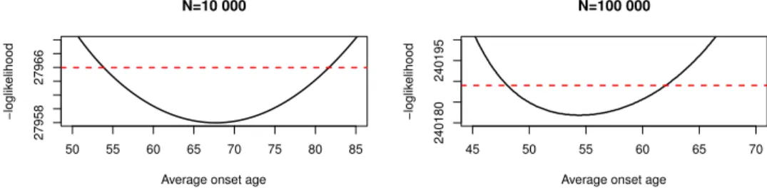
When we studied the profile likelihood of the onset, it became clear that multiple parameters can maximize the likelihood and that the confidence region is vast. This can be seen in Figure 2, where we plot the negative loglikelihood fixing𝜉and𝜆2to the estimated values and variating𝜆1. The confidence region for the average onset age1/𝜆2 is [49.31;71.67] for the small data set and [48.7;61.07] for the large one.

(8)

The reason behind this large region is the exponential onset, that is very dense near 0 and decays quickly. Since we only start observing patients older than 𝑡_min=40 years old and follow them up for 10 years, there is no information about the densest interval(0, 𝑡_min), it is difficult for the model to estimate𝜆1 for a small sample size. The dissimilarity to the actual density within the observation period is not detectable. Increasing the sample size allows better estimation of the parameters although the confidence region is still sizable. In this scenario, one can think of the disease progression as a flow process with the parameters controlling the rate of flow between states, accordingly, there are different flow rates which generate the same output.

50 55 60 65 70 75 80 85

2795827966

N=10 000

Average onset age

−loglikelihood

45 50 55 60 65 70

240180240195

N=100 000

Average onset age

−loglikelihood

Figure 2. Profile likelihood of the average onset for the small data (left) and the large one (right), the red line is the critical threshold

for the likelihood based confidence region.

Another observation is the very strong negative correlation between the sensitivity and the sojourn time estimators (the correlation measured using the observed Fisher information matrix between 𝑏0 and 𝜉 is around −0.8). Although they are assumed independent in the model, screening acts as a censoring mechanism, once a case is detected, the rest of its sojourn time cannot be observed. What happens then is that the model preserves a good fit in one of two ways, the first is by re- turning a high sensitivity estimate and a low sojourn time meaning that cases stay a short time in the preclinical state but participation in a screen leads to detection with a high probability. The second is by combining a high sojourn time estimate with a low sensitivity, meaning that cases will stay for a longer time in the preclinical state, therefore having multiple chances to participate in a screen, with screens having a low probability of detection. We observed this negative correlation in all of our parameterizations.

4.1.2. Lognormal onset

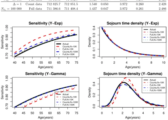
The results for a lognormally distributed onset time and an exponentially distributed sojourn time are presented in Table 2, plots for the sensitivity and the sojourn time are presented in the top part of Figure 3.

For (𝑁𝑡1 = 10 000), the sensitivity and onset parameters are substantially biased when using the count data, while using the full model results in more accurate estimates. Increasing the number of participants to 100 000 (second block), we

(9)

noticed a slight improvement in the performance of the count based model and a significant improvement when using the full model.

Table 2. Estimates of the sensitivity (𝑏0, 𝑏1), onset (𝜇, 𝑠) and sojourn time (𝜆)parameters for a lognormal𝑋 and an exponential𝑌.

-Loglikelihood Sensitivity Preclinical intensity Sojourn time

Maximum Actual 𝑏0 𝑏1 𝜇 𝑠 𝜆

Actual 1.4 0.05 3.971 0.267 2.5

∆ = 1 Count data 71 777.0 71 786.6 1.971 0.081 3.969 0.253 2.236 𝑁𝑡1=10 000 Full data 71 647.6 71 652.7 1.529 0.061 3.969 0.257 2.423

∆ = 1 Count data 712 825.7 712 851.5 1.540 0.050 3.972 0.260 2.428 𝑁𝑡1=100 000 Full data 711 386.6 711 408.4 1.437 0.047 3.972 0.261 2.486

40 45 50 55 60 65 70 75

0.700.800.901.00

Sensitivity (Y~Exp)

Age(years)

Sensitivity

Actual Counts,N=10K Full,N=10K Counts,N=100K Full,N=100K

0 2 4 6 8 10

0.00.10.20.30.4

Sojourn time density (Y~Exp)

Age(years)

Density

40 45 50 55 60 65 70 75

0.700.800.901.00

Sensitivity (Y~Gamma)

Age(years)

Sensitivity

0 1 2 3 4 5 6

0.00.20.4

Sojourn time density (Y~Gamma)

Age(years)

Density

Figure 3. Sensitivity and the sojourn time density for lognormal 𝑋 and exponential𝑌 (top), lognormal𝑋 and gamma𝑌 (bottom).

In order to evaluate the performance of the model and create reliable confidence intervals for the estimators for the small dataset, we ran the simulator 50 times and estimated the parameters based on both models. We also calculated the likelihood based confidence regions. The resulting confidence intervals are displayed in Table 3. We noticed that the intervals based on the full model are tighter than those of the count based ones. Besides, the likelihood-based confidence intervals for the sensitivity parameters 𝑏0 and𝑏1 are larger than those based on the simulation. That is not the situation for the mean sojourn time intervals, where the likelihood-based intervals are tighter. The strong negative correlation between the sojourn time and the sensitivity creates a multi-centered confidence region for the

(10)

sojourn time. Since the likelihood based intervals are built around one center, they appear tighter than they actually are.

Table 3. Likelihood based and simulation based confidence intervals for the count based and the full models.

Count based model Full model

Simulations Likelihood Simulations Likelihood 𝑏0 [1.425; 1.925] [1.612; 2.418] [1.346; 1.783] [1.296; 1.786]

𝑏1 [0.0294; 0.0808] [0.0219; 0.134] [0.0314; 0.0672] [0.0221; 0.101]

1/𝜆 [2.200; 2.663] [2.095; 2.392] [2.298; 2.590] [2.185; 2.302]

4.2. Gamma sojourn time

For a lognormal onset and a gamma distributed sojourn time, the estimates are presented in Table 4, plots for the sensitivity and the sojourn time are shown in the bottom part of Figure 3.

For the small data set, the sensitivity estimates are biased under both models (bottom left part of Figure 3). Besides, estimates of the sojourn time parameters for both models are strange at first glance. However, these parameters result in acceptable estimates of the mean sojourn time, although the sojourn time variance is substantially underestimated in both cases.

Table 4. Estimates of the sensitivity (𝑏0, 𝑏1), onset (𝜇, 𝑠) and sojourn time (𝜆)parameters for a lognormal𝑋 and gamma𝑌.

-Loglikelihood Sensitivity Preclinical intensity Sojourn time

Maximum Actual 𝑏0 𝑏1 𝜇 𝑠 𝛼 𝛽 E(𝑌) V(𝑌)

Actual 1.4 0.05 3.971 0.267 6.25 2.5 2.5 1

∆ = 1 Count data 68 069.8 68 077.4 1.114 0.045 3.970 0.261 10.252 3.940 2.602 0.661 𝑁𝑡1=10 000 Full data 68 040.3 68 047.3 1.181 0.047 3.970 0.261 8.407 3.259 2.580 0.792

Moving on to the second block (larger dataset), both models perform well and their results are very close. However, the estimates of the sojourn time variance are still biased, the plots in Figure 3 show that estimated sojourn time density based on the full model is very close to the actual one although a slight bias is observed.

In general, the model seems to perform well in this case, with some slight bias in the sensitivity and the variance of the sojourn time. However, to test the reliability of our confidence sets, we fixed all the parameters to their estimated values (𝑁𝑡1 =100 000) and calculated the profile likelihood for different𝛼 and𝛽.

The contour plot can be seen in Figure 4, which clearly shows that the likelihood- based confidence region (black region) contains a substantial part of the line 𝛼= 2.5𝛽.

(11)

7e+05

7e+05 750000

8e+05 850000

5 10 15 20

Alpha)

Beta

−loglikelihood (0,6.77e+05]

(6.77e+05,6.78e+05]

(6.78e+05,6.8e+05]

(6.8e+05,6.83e+05]

(6.83e+05,6.87e+05]

(6.87e+05,6.91e+05]

(6.91e+05,6.96e+05]

(6.96e+05,7.03e+05]

(7.03e+05,7.12e+05]

(7.12e+05,7.23e+05]

(7.23e+05,7.38e+05]

(7.38e+05,7.57e+05]

(7.57e+05,7.83e+05]

(7.83e+05,8.18e+05]

(8.18e+05,8.78e+05]

(8.78e+05,1.19e+06]

Figure 4. Contour plot of the loglikelihood (𝑁𝑡1= 100000)using the estimated sensitivity and onset parameters and variating𝛼and 𝛽. The black region represents the likelihood based confidence re-

gion.

The figure shows that the likelihood is near constant in the neighborhood of the line 𝛼 = 2.5𝛽. In this neighborhood, the expected value of the gamma distributed mean sojourn time is almost constant (𝛼/𝛽 = 2.5), however, there is a great variation of the variance (𝛼/𝛽²), which does not affect the likelihood, this essentially means that the variance could be much larger or smaller and still fall in the likelihood based confidence region, with the noise in the data determining where the center of that region is. The model is then not able to estimate the variance of the sojourn time under this setup.

To further test the ability of the model to estimate the sojourn time variance, we generated a dataset (𝑁𝑡1 = 100 000, 𝐾 = 10) based on 𝛼= 100 and 𝛽 = 10 resulting in a mean sojourn time of 10 years and a variance of 1. In this case, fitting a constant sojourn time of 10 years results in a -loglikelihood of 928 675.1, almost identical to the -loglikelihood based on the original parameters (928 674.3). This means that for large enough parameters 𝛼0 and𝛽0 where 𝛼0/𝛽0 = 10, the model retains a good fit regardless of the variance, showing that there are infinitely many parameters maximizing the likelihood. Hence, the model is not able to estimate the variance of the sojourn time when∆ is too small since the tail of the sojourn time cannot be observed due to screening.

A larger inter-screening interval means that there are fewer opportunities for an individual to participate in a screening exam, thus it will lead to a high number of clinically detected (interval) cases and therefore more information about the sojourn time tail, we investigate this question in the next subsection.

(12)

4.3. Larger inter-screening time

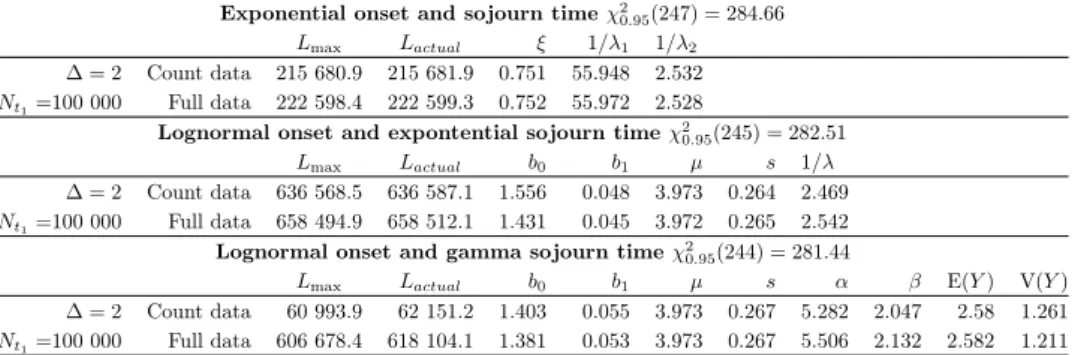
In order to study the effect of a larger inter-screening time, we used the same disease progression data of size 100 000 and ran a screening program consisting of 5 screens with 2 years between each screen. The results are presented in Table 5.

The models perform well in general, the estimates are more accurate than the case where the inter-screening time is one year.

Table 5. Estimates of the process governing parameters for an inter-screening time of 2 years.

Exponential onset and sojourn time𝜒²_0.95(247) = 284.66

𝐿_max 𝐿𝑎𝑐𝑡𝑢𝑎𝑙 𝜉 1/𝜆1 1/𝜆2

∆ = 2 Count data 215 680.9 215 681.9 0.751 55.948 2.532 𝑁𝑡1=100 000 Full data 222 598.4 222 599.3 0.752 55.972 2.528

Lognormal onset and expontential sojourn time𝜒²_0.95(245) = 282.51

𝐿max 𝐿𝑎𝑐𝑡𝑢𝑎𝑙 𝑏0 𝑏1 𝜇 𝑠 1/𝜆

∆ = 2 Count data 636 568.5 636 587.1 1.556 0.048 3.973 0.264 2.469 𝑁𝑡1=100 000 Full data 658 494.9 658 512.1 1.431 0.045 3.972 0.265 2.542 Lognormal onset and gamma sojourn time𝜒²_0.95(244) = 281.44

𝐿_max 𝐿𝑎𝑐𝑡𝑢𝑎𝑙 𝑏0 𝑏1 𝜇 𝑠 𝛼 𝛽 E(𝑌) V(𝑌)

4.4. Misspecifications

Since it is not possible to observe neither the exact onset nor the sojourn time of breast cancer, there is a possibility that one may falsely assume the sensitivity to be constant or model the process with an incorrect distribution. In order to investigate the performance of the model under these false assumptions, we first force the sensitivity to be constant by fixing𝑏1= 0.

To investigate the performance of the model when one misspecifies the distribution of the sojourn time, the model is run on the data generated by a known distribution, while using an incorrect distribution to model the sojourn time.

4.4.1. Constant sensitivity

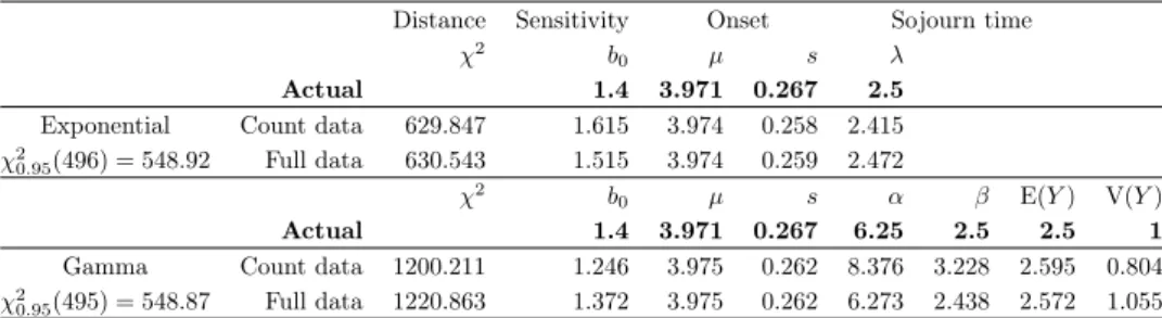
Let us first use a constant sensitivity (𝑏1 = 0) and fit the count based and the full model on the data (𝑁𝑡1 =100 000 and∆ = 1) generated by a lognormal onset combined with an exponential and gamma sojourn times. The results can be seen in Table 6.

It seems that forcing the sensitivity to be constant does not have a large effect on the estimates for an exponentially distributed sojourn time. However, the 𝜒²- distance in both cases does not fall in the acceptance region.

In the second block of the table, where the sojourn time is gamma distributed, a bias can be observed in the variance of the sojourn time but the full model still performs quite well regardless of the false assumption. We also noticed that the

(13)

𝜒²−distance for both models is extremely large and is way outside the acceptance region.

Table 6. Estimates of the sensitivity (𝑏0), onset (𝜇, 𝑠) and sojourn time (𝜆)parameters when forcing a constant sensitivity (𝑏1= 0).

Distance Sensitivity Onset Sojourn time

𝜒² 𝑏0 𝜇 𝑠 𝜆

Actual 1.4 3.971 0.267 2.5

Exponential Count data 629.847 1.615 3.974 0.258 2.415 𝜒²_0.95(496) = 548.92 Full data 630.543 1.515 3.974 0.259 2.472

𝜒² 𝑏0 𝜇 𝑠 𝛼 𝛽 E(𝑌) V(𝑌)

Actual 1.4 3.971 0.267 6.25 2.5 2.5 1

Gamma Count data 1200.211 1.246 3.975 0.262 8.376 3.228 2.595 0.804 𝜒²_0.95(495) = 548.87 Full data 1220.863 1.372 3.975 0.262 6.273 2.438 2.572 1.055

4.4.2. Incorrect distribution

In order to investigate the effect of misspecifying the sojourn time distribution, we used an exponential distribution to model the data generated by a gamma sojourn time (∆ = 1and𝑁𝑡1=100 000). The results are displayed in Table 7.

Table 7. Estimates of the key parameters when misspecifying the sojourn time distribution.

Fitting an exponential sojourn time 𝜒²_0.95(497) = 549.97

𝑌 ∼ 𝜒² 𝑏0 𝑏1 𝜇 𝑠 1/𝜆

Gamma Count data 8946.79 2.546 0.154 4.006 0.296 3.632 Full data 9048.17 2.093 0.119 4.008 0.3 3.827 When an exponential distribution is fitted to data generated by a gamma sojourn time, the model does not perform well, the 𝜒²-distances are enormous for both models. The estimates for the mean sojourn time are very high and both sensitivity and preclinical intensity parameters are also highly overestimated. This is highly problematic as the exponential distribution is the most used one in the literature.

The likely reason behind the high mean sojourn time estimate is the inability of the exponential distribution, which is a one parameter family, to fit the shape of a two parameter distribution (gamma). We also noticed that in this case, the count based model has a slightly better mean sojourn time estimate than that of the full model, since adding the exact time of diagnosis forces the exponential distribution to fit a density with a peak leading to worse results. The multicorrelation explains the estimates for the sensitivity and the onset, the model adjusts by increasing the sensitivity of screens and onset age to compensate for the inability of the exponential distribution to fit the data.

(14)

5. Consequences for previous results

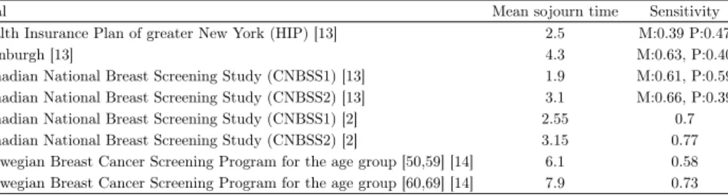
The estimates of the mean sojourn time and the sensitivity in some famous clinical trials are shown in Table 8. One immediately notices the discrepancy between the estimates, there are completely different estimates based on the same data set but using different assumptions. We aim to discuss the reasons behind this inconsistency.

Table 8. Sojourn time and sensitivity estimates (M: mammography, P: physical exam) for some clinical trials.

Trial Mean sojourn time Sensitivity

Health Insurance Plan of greater New York (HIP) [13] 2.5 M:0.39 P:0.47

Edinburgh [13] 4.3 M:0.63, P:0.40

Canadian National Breast Screening Study (CNBSS1) [13] 1.9 M:0.61, P:0.59 Canadian National Breast Screening Study (CNBSS2) [13] 3.1 M:0.66, P:0.39

Canadian National Breast Screening Study (CNBSS1) [2] 2.55 0.7

Canadian National Breast Screening Study (CNBSS2) [2] 3.15 0.77

Norwegian Breast Cancer Screening Program for the age group [50,59] [14] 6.1 0.58 Norwegian Breast Cancer Screening Program for the age group [60,69] [14] 7.9 0.73

Chen et al. [2] used a stable disease approach and used the gamma distribution to model the sojourn time of breast cancer. They applied their model on the CNBSS data. They modeled the 40–49-year-old and 50–59-year-old cohorts separately.

The sensitivity is assumed to be constant, we have shown that forcing a constant sensitivity barely affects the rest of the parameters. However, assuming the onset to be independent of age is not likely to hold true.

In the approach used by Wu et al [16], they used constraints on the sojourn time, the preclinical intensity, as well as the sensitivity when maximizing the likelihood.

In other words, they run MCMC simulation on a bounded area to find a maximum, which could force a convergence to a local maximum. They also introduced using a loglogistic sojourn time to model the sojourn time, which has similar shape to the lognormal distribution but has heavier tails, it also has desirable survival rate properties.

To check the model performance under a loglogistic sojourn time, we ran the simulator based on a scale𝛼= 2.336and a shape𝛽= 4.951, to generate a data set of size𝑁𝑡1 = 100 000, the defined values lead to a mean sojourn time of 2.5 years and unit variance. After running the count based and the full model, we noticed that the estimates are generally accurate and the performance of the model is similar to the gamma sojourn time case. That being said, the variance of the sojourn time is also hard to estimate in this case.

Furthermore, we also used the loglogistic sojourn time to model the data based on the exponential and gamma distributions. For the exponential data, the count based model performed well, with acceptable estimates. However, the full model fails to estimate the parameters (estimated mean sojourn time of 3.41 years), this is caused by the inability of the loglogistic distribution to fit the exponential shape.

(15)

On the other hand, when fitting the model to data generated by a gamma sojourn time, the results are almost indifferentiable to actually fitting a gamma sojourn time. Even the likelihood based on the full models are almost identical, with a -loglikelihood of 676 562.9 when fitting a gamma distribution and 676 564.9 when fitting a loglogistic one. This means that there is no difference between the fit of the two distributions and one is not able to differentiate between them.

Regarding the conflicting results of the CNBSS1 studies, [13] estimated the sensitivity for Mammography(M) and physical examination(P) independently, their mean sojourn time estimate for the CNBSS1 trial is 1.9 years, significantly lower than the estimate of [2] of 2.55 years, the multicorrelation and different sojourn time distributions is possibly the reason behind the difference in the estimates.

A two parameters (entry–exit) Markov chain model is used by [3], assuming that the incidence rate𝜆1 and the rate of transition from the preclinical state to the clinical one 𝜆2 are both constants. When this method is applied to the data from the Swedish two-county study of breast cancer screening in the age group 70-74, the resulting estimate for the mean sojourn time is 2.3 years. Although the model is very flexible in the sense that symptomatic data is not needed, we have shown that the parameters are not identifiable in this setup.

Weedon-Fekjaer et al. used a weighted non-linear least-square regression estimates based on a three step Markov chain model, then performed sensitivity anal- ysis to determine the possible impact of opportunistic screening between regular screening rounds. Mean sojourn time and sensitivity were estimated by non-linear least square regression, using number of cancer cases at screening and in the interval between screening examinations. Mean sojourn time was estimated as 6.1 (95%

confidence interval [CI] 5.1-7.0) years for women aged 50-59 years, and 7.9 years (95% CI 6.0-7.9) years for those aged 60-69 years, sensitivity was estimated as 58%

(95% CI 52-64 %) and 73 % (67-78 %), respectively. We suspect that the high sojourn time estimate is a consequence of the choice of the sojourn time distribution, as we have shown earlier, using the exponential distribution to model a sojourn time having a different distribution results in a very high sojourn time estimate.

Their findings also suggest that sensitivity is lower than in other programs as well as a higher mean sojourn time, but we believe it to be a direct consequence of the correlation between the two parameters.

6. Summary

Summing up our findings, we can state that the current models are very sensitive to the underlying assumptions. One should take great care of using such an approach, and multiple trials with different models are needed before in order to get reliable results. One way to solve this problem might be to include more information in the model to stabilize the results such as tumor growth shape and tumor size [6, 7]. Under an exponential onset and sojourn time, the parameters are not identifiable for a small sample, the acceptance region is sizable and data before the

(16)

first screen is needed to stabilize the results. On the other hand, under a lognormal onset and an exponential sojourn time, the model performs much better and estimates are generally accurate. Overall, the model performs well in this case, we noticed that the full model performs much better than the count-based one.

Nonetheless, it would be wiser to apply the gamma model for the sojourn time, as it is much more flexible and it can be reduced to the exponential distribution in case the shape estimate is close to one.

The performance of the model is satisfactory for a gamma sojourn time, however estimates of the variance of the sojourn time are quite biased. A larger inter- screening interval improves the variance estimate since it allows observing the tail of the sojourn time before censoring (screening). But of course medical considerations might be more important in practice.

We also observed a high correlation between the parameters under all parameterizations. Consequently, the obtained variances of the estimators are not as reliable as we might think. On the other hand, including the exact date of diagnosis leads to more accurate estimates for a small sample size and a more compact acceptance region. We recommend applying both the count and the full model, and if they give inconsistent results, then misspecification might be the reason for this. The likelihood based on the full model is much more sensitive to small shifts in the parameters, since it will be magnified through the product of the likelihood of symptomatic cases. That is not the case with the count-based model.

Higher inter-screening intervals result in less accurate estimates for the sensitivity but better sojourn time variance estimates. We also noticed that the 𝜒² distance of the count-based model was always smaller than that of the full one, although the latter allows for better estimates. Since maximizing the count-based likelihood is equivalent to minimizing the𝜒²-distance, this is a sign of over-fitting.

Nonetheless, the 𝜒²-distance can serve as good indicator for misspecification or incorrect assumptions.

References

[1] R. Byrd,P. Lu,J. Nocedal,C. Zhu:A limited memory algorithm for bound constrained optimization, SIAM Journal of Scientific Computing 16 (1995), pp. 1190–1208,issn: 1064- 8275,

doi:https://doi.org/10.1137/0916069.

[2] Y. Chen,G. Brock,D. Wu:Estimating key parameters in periodic breast cancer screening—Application to the Canadian National Breast Screening Study data, Cancer Epidemi- ology 34.4 (2010), pp. 429–433,issn: 1877-7821,

doi:https://doi.org/10.1016/j.canep.2010.04.001.

[3] S. W. Duffy,H.-H. Chen, L. Tabar,N. E. Day:Estimation of mean sojourn time in breast cancer screening using a Markov chain model of both entry to and exit from the preclinical detectable phase, Statistics in Medicine 14.14 (1995), pp. 1531–1543,

doi:https://doi.org/10.1002/sim.4780141404.

[4] D. Eddelbuettel,J. J. Balamuta:Extending extitR with extitC++: A Brief Introduction to extitRcpp, PeerJ Preprints 5 (2017), e3188v1,issn: 2167-9843,

doi:https://doi.org/10.7287/peerj.preprints.3188v1.

(17)

[5] T. Hahn:Cuba—a library for multidimensional numerical integration, Computer Physics Communications 168.2 (2005), pp. 78–95,issn: 0010-4655,

doi:https://doi.org/10.1016/j.cpc.2005.01.010.

[6] A. Hijazy,A. Zempléni:Gamma Process-Based Models for Disease Progression, Methodol Comput Appl Probab (2020),

doi:https://doi.org/10.1007/s11009-020-09771-4.

[7] A. Hijazy,A. Zempléni:Optimal inspection for randomly triggered hidden deterioration processes, Quality and Reliability Engineering International (2020),

doi:https://doi.org/10.1002/qre.2707.

[8] S. J. Lee,M. Zelen:Scheduling Periodic Examinations for the Early Detection of Disease:

Applications to Breast Cancer, Journal of the American Statistical Association 93.444 (1998), pp. 1271–1281,

doi:https://doi.org/10.1080/01621459.1998.10473788.

[9] G. Parmigiani,S. Skates:Estimating distribution of age of the onset of detectable asymptomatic cancer, Mathematical and Computer Modelling 33.12 (2001), pp. 1347–1360,issn:

0895-7177,

doi:https://doi.org/10.1016/S0895-7177(00)00320-4.

[10] P. C. Prorok:The theory of periodic screening II: doubly bounded recurrence times and mean lead time and detection probability estimation, Advances in Applied Probability 8.3 (1976), pp. 460–476,

doi:https://doi.org/10.2307/1426139.

[11] S. P. Shapiro S. Venet W.,V. L.:Periodic Screening for Breast Cancer. The Health Insurance Plan Project,1963–1986, and its Sequelae, 1988.

[12] Y. Shen, M. Zelen:Parameteric estimation procedures for screening programmes: Sta- ble and non stable disease models for multimodality case findings, Biometrika 86.3 (1999), pp. 503–515.

[13] Y. Shen,M. Zelen:Screening Sensitivity and Sojourn Time From Breast Cancer Early Detection Clinical Trials: Mammograms and Physical Examinations, Journal of Clinical Oncology 19.15 (2001), pp. 3490–3499,

doi:https://doi.org/10.1200/JCO.2001.19.15.3490.

[14] H. Weedon-Fekjær,L. J. Vatten,O. O. Aalen,B. Lindqvist,S. Tretli:Estimating mean sojourn time and screening test sensitivity in breast cancer mammography screening:

new results, Journal of Medical Screening 12.4 (2005), pp. 172–178, doi:https://doi.org/10.1258/096914105775220732.

[15] S. S. Wilks:The Large-Sample Distribution of the Likelihood Ratio for Testing Composite Hypotheses, Ann. Math. Statist. 9.1 (1938), pp. 60–62,

doi:https://doi.org/10.1214/aoms/1177732360.

[16] D. Wu,G. L. Rosner,L. Broemeling:MLE and Bayesian Inference of Age-Dependent Sensitivity and Transition Probability in Periodic Screening, Biometrics 61.4 (2005), pp. 1056–

1063,

doi:https://doi.org/10.1111/j.1541-0420.2005.00361.x.

[17] M. Zelen,M. Feinleib:On the theory of screening for chronic diseases, Biometrika 56.3 (1969), pp. 601–614,

doi:https://doi.org/10.1093/biomet/56.3.601.