Tropical Dominating Sets in Vertex-Coloured Graphs
J.-A. Anglès d’Auriac
1, Cs. Bujtás
2, A. El Maftouhi
1, M. Karpinski
3, Y. Manoussakis
1, L. Montero
1, N. Narayanan
1, L. Rosaz
1,
J. Thapper
4, Zs. Tuza
2,51 Université Paris-Sud, L.R.I., Bât. 650, 91405 Orsay Cedex, France.
2 Department of Computer Science and Systems Technology, University of Pannonia, 8200 Veszprém, Egyetem u. 10, Hungary.
3 University of Bonn, Department of Computer Science, Friedrich-Ebert-Allee 144, 53113 Bonn, Germany.
4 Université Paris-Est, Marne-la-Vallée, LIGM, Bât. Copernic, 5 Bd Descartes, 77454 Marne-la-Vallée Cedex 2, France.
5 Alfréd Rényi Institute of Mathematics, Hungarian Academy of Sciences, 1053 Budapest, Reáltanoda u. 13–15, Hungary.
angles@lri.fr, bujtas@dcs.uni-pannon.hu, hakim.maftouhi@orange.fr, marek@cs.uni-bonn.de, yannis@lri.fr, lmontero@lri.fr,
narayana@gmail.com, rosaz@lri.fr, thapper@u-pem.fr, tuza@dcs.uni-pannon.hu
Abstract
Given a vertex-coloured graph, a dominating set is said to be tropical if every colour of the graph appears at least once in the set. Here, we study minimum tropical dominating sets from structural and algorithmic points of view. First, we prove that the tropical dominating set problem is NP-complete even when restricted to a simple path. Then, we establish upper bounds related to various parameters of the graph such as minimum degree and number of edges. We also give an optimal upper bound for random graphs. Last, we give approximability and inapproximability results for general and restricted classes of graphs, and establish a FPT algorithm for interval graphs.
Keywords: Dominating set, Vertex-coloured graph, Approximation, Random graphs
1 Introduction
Vertex-coloured graphs are useful in various situations. For instance, the Web graph may be considered as a vertex-coloured graph where the colour of a vertex represents the content of the corresponding page (red for mathematics, yellow for physics, etc). Given a vertex-coloured graphGc, a subgraph Hc (not necessarily induced) ofGc is said to be tropical if and only if each colour ofGc appears at least once in Hc. Potentially, any kind of usual structural problems (paths, cycles, independent and dominating sets, vertex covers, connected components, etc.) could be studied in their tropical version. This new tropical concept is close to, but quite different from, the colourful concept used for paths in vertex-coloured graphs [1, 26, 27]. It is also related to (but again different from) the concept ofcolour patterns used in bio-informatics [18]. Here, we study minimum tropical dominating sets in vertex-coloured graphs. Some ongoing work on tropical connected components, tropical paths and tropical homomorphisms can be found in [13, 14, 19]. A general overview on the classical dominating set problem can be found in [23].
arXiv:1503.01008v3 [cs.DM] 18 Jan 2016
Throughout the paper letG= (V, E) denote a simple undirected non-coloured graph. Letn=|V| andm=|E|. Given a set of coloursC={1, ..., c},Gc= (Vc, E) denotes a vertex-coloured graph where each vertex has precisely one colour fromC and each colour ofC appears on at least one vertex. The colour of a vertexxis denoted byc(x). A subset S⊆V is adominating set ofGc (or ofG), if every vertex either belongs toS or has a neighbour inS. Thedomination number γ(Gc) (γ(G)) is the size of a smallest dominating set ofGc (G). A dominating setS ofGc is said to betropical if each of thec colours appears at least once among the vertices ofS. Thetropical domination number γt(Gc) is the size of a smallest tropical dominating set ofGc. Arainbow dominating setofGcis a tropical dominating set with exactlyc vertices. More generally, ac-element set with precisely one vertex from each colour is said to be arainbow set. We letδ(Gc) (respectively ∆(Gc)) denote the minimum (maximum) degree ofGc. When no confusion arises, we writeγ, γt, δand ∆ instead ofγ(G),γt(Gc),δ(Gc) and ∆(Gc), respectively. We use the standard notationN(v) for the (open) neighbourhood of vertexv, that is the set of vertices adjacent tov, and writeN[v] =N(v)∪ {v}for its closed neighbourhood. The set and the number of neighbours ofv inside a subgraphH is denoted byNH(v) and bydH(v), independently of whetherv is inH or inV(Gc)−V(H). Although less standard, we shall also write sometimes v∈Gc to abbreviatev∈V(Gc).
Note that tropical domination in a vertex-coloured graphGccan also be interpreted as “simultaneous domination” in two graphs which have a common vertex set. One of the two graphs is the non-coloured Gitself, the other one is the union of cvertex-disjoint cliques each of which corresponds to a colour class inGc. The notion of simultaneous dominating set1was introduced by Sampathkumar [32] and independently by Brigham and Dutton [9]. It was investigated recently by Caro and Henning [10] and also by further authors. Remark thatδ≥1 is regularly assumed for each factor graph in the results of these papers that is not the case in the present manuscript, as we do not forbid the presence of one-element colour classes.
The Tropical Dominating Set problem (TDS) is defined as follows.
Problem 1. TDS
Input: A vertex-coloured graph Gc and an integerk≥c.
Question: Is there a tropical dominating set of size at most k?
The Rainbow Dominating Set problem (RDS) is defined as follows.
Problem 2. RDS
Input: A vertex-coloured graph Gc.
Question: Is there a rainbow dominating set?
The paper is organized as follows. In Section 2 we prove that RDS is NP-complete even when graphs are restricted to simple paths. In Section 3 we give upper bounds forγtrelated to the minimum degree and the number of edges. We give upper bounds for random graphs in Section 4. In Section 5 we give approximability and inapproximability results for TDS. We also show that the problem is FPT (fixed-parameter tractable) on interval graphs when parametrized by the number of colours.
2 NP-completeness
In this section we show that the RDS problem is NP-complete. This implies that the TDS problem is NP-complete too.
Theorem 2.1. The RDS problem is NP-complete, even when the input is restricted to vertex-coloured paths.
Proof. Clearly the RDS problem is in NP. The reduction is obtained from the 3-SAT problem. Let (I, Y) be an instance of 3-SAT whereI = (l1∨l2∨l3)∧(l4∨l5∨l6)∧. . .∧(lX−2∨lX−1∨lX) is a
1Also known under the names ‘factor dominating set’ and ‘global dominating set’ in the literature.
collection ofτ=X/3 clauses on a finite setY ={y1, . . . , ym}of boolean variables. From this instance, we will define a vertex-coloured pathP such thatP contains a rainbow dominating set if and only if (I, Y) is satisfiable.
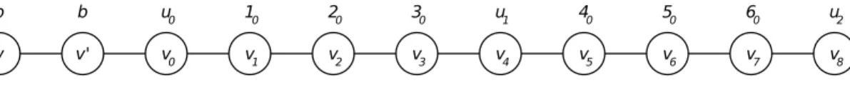
In order to defineP, we first construct a segmentP0=vv0v0v1. . . v4τ, and we colour its vertices as follows. Verticesvandv0 are coloured black. Verticesv0, v4, v8, . . . , v4τ−4, v4τ are each coloured with a unique colour. The remaining vertices, that will be henceforth calledclausal, are coloured fromv1 to v4τ−1 with colours 10,20,30, . . . , X0. Figure 1 shows P0 ifX= 6.
Figure 1: Example ofP0whenX = 6
Next, we define a number of gadgets as follows. If a pair of literalsli andlj satisfies thatli=lj, we say thatlj isantithetic toli. For each literal li, i= 1, . . . , X, we consider the list of all literals li1, li2, . . . , liki that are antithetic toli. Now, to each literallif,f = 1, . . . , ki, we associate aconstraint gadget wi,if on five vertices defined as follows. Vertex Ais an artificial one and is coloured with a unique colour. VertexP is thepositiveone of the gadget, it corresponds to literallibeing true and has colourif. ThemiddlevertexM is coloured with black. VertexN is thenegative one, it corresponds toli being false and has colourif−1. VertexLis thelink vertex and represents the relation between li andlif. Ifi < if, thenL is coloured with colour ci,if, otherwise, with colourcif,i. See Figure 2.
Finally, in order to obtain pathP, we concatenate all these gadgets toP0 in a serial manner and we close the path with a final vertexF of a unique colour. Clearly, this construction is polynomial as we haveO(X2) gadgets.
Figure 2: A constraint gagdetwi,if (wherei < if)
We first prove the"if case". Consider an assignment to the variablesy1, . . . , ym that satisfies the 3-SAT instance. From this assignment we obtain a rainbow dominating setDforP as follows:
1. We addvand every vertex of a unique colour toD.
2. For each true literalli, we add the clausal vertex of colouri0 toDand for allf = 1, . . . , ki (if any), we add the positive vertexP and the link vertexLofwi,if toD.
3. For each false literalli and all f = 1, . . . , ki (if any), we add the negative vertexN ofwi,if toD.
4. If there are vertices with some colour still not present inD, we add them to the set.
We can check that each colour is present exactly once inD. In fact, this conclusion is straightforward for black colour, for every unique colour and for each colourif. For the colour on the link vertexLof a gadgetwi,j, as literalsli andlj are antithetic, then exactly one of them is true, so it stands that either ci,j is present once inDifi < j, or cj,i otherwise.
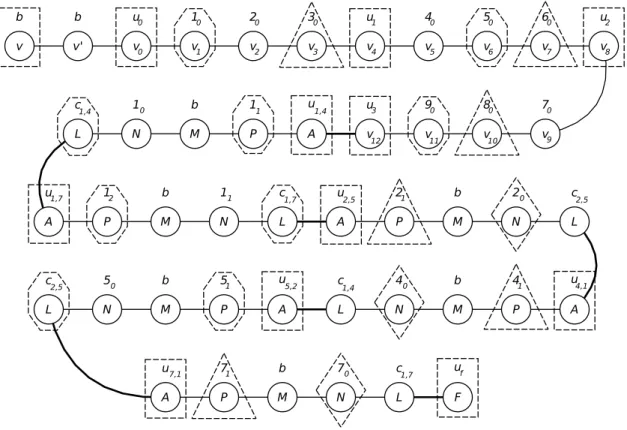
We show now that Dis a dominating set. Observe first that v0 is dominated by v (and also by v0). Then, as every clause contains at least one true literal, every clausal vertex is either inDor has some neighbour inD. Last, every constraint gadget has either its negative vertex or both its positive and link vertex inD. In both cases, all vertices of the gadget are covered byD. Therefore D is a rainbow dominating set as claimed. An example of the construction ofP and its corresponding rainbow dominating setDfor an arbitrary assignment to the variables is shown in Figure 3.
Figure 3: Construction ofP for the formula (y1∨y2∨y3)∧(y1∨y2∨y3)∧(y1∨y3∨y4) where P =P0w1,4w1,7w2,5w4,1w5,2w7,1F. The colour of the vertices is shown on top of them and the thick edges represent the division of the gadgets. Vertices surrounded by dotted~,8,♦and are the ones taken by the steps 1,2,3 and 4, respectively, to obtain the rainbow dominating setDcorresponding to the assignmenty1=y2=y4=T rueandy3=F alse. Note that the step 4 is not needed for the set to be dominating but it is to become rainbow.
We now prove the "only if" case. Given the path P constructed as before, let D be a rainbow dominating set forP. We consider first a partial assignment where for every clausal vertex of colour i0 that is in D, we assign the value to the corresponding variable such that li is true. Suppose by contradiction that this assignment method leads to some incoherences, that is, some variable ends up being assigned both true and false. It implies thatDcontains two clausal vertices of colouri0and j0, respectively, such thatli andlj are antithetic. Suppose without loss of generality thati < j. Asli and lj are antithetic, there exist two gadgetswi,if,if =j, andwj,j
f0,jf0 =i, where the link vertices are both colouredci,j (asi < j). We will show that both of those vertices are inDlead to a contradiction.
Considerwi,if (a similar proof works forwj,jf0).
Suppose first that f = 1. If L does not belong to D, then N must be in D as M being black, cannot belong toDsinceDmust already contain eithervorv0 that are also coloured black. This is a contradiction since the colour ofN isi0 andDalready contains the clausal vertex on that colour.
ThereforeLbelongs toD.
Suppose next thatf >1. By the same argument as before, ifLdoes not belong toDthenN must be inD. As the colour ofN is if−1, then the vertexP of wi,if−1 cannot belong toDsince it has the same colour. Therefore, asDmust dominate the vertexM of wi,if−1, we have that the vertexN on colourif−2 ofwi,if−1 belongs toD. Following the same argument, we have that the negative vertexN belongs toDfor eachwi,ik, k=f, . . . ,1. This is a contradiction since the vertexN ofwi,i1 has colour i0andDalready contains the clausal vertex on that colour. ThereforeL belongs toD.
As the same reasoning holds forwj,jf0 as well,D contains two vertices of colourci,j. This is a contradiction to the hypothesis that D is rainbow. Hence our partial assignment is coherent. We complete the assignment by setting to true every unassigned variable.
Now, it remains to see that the obtained assignment satisfies the 3-SAT instance. Indeed, as every clausal vertex is covered byD, then for every clause we have one literal who was assigned to true, that is, the assignment is a solution to the 3-SAT instance. This completes the argument and the proof of the theorem.
3 Upper Bounds
We begin with an easy observation which intends to avoid some trivial technical distinctions later on.
Proposition 3.1. If Gc is a vertex-coloured graph with c colours onn vertices, and δ(Gc)≥n−c, then every rainbow set is a rainbow dominating set ofGc. As a consequence, γt(Gc) =c holds.
Proof. LetDbe any rainbow set, andv∈V(Gc)−Dany vertex. Then|N[v]|≥δ(Gc) + 1≥n−c+ 1 =
|V(Gc)−D|+1, thus Ddominatesv.
Without further reference to this proposition, throughout the text below, we shall disregard whether or not any proof works for graphs of minimum degree at leastn−c, because we know the tropical domination number of those graphs exactly.
Proposition 3.2. For any graph Gc,γt≤γ+c−1. Furthermore, there are extremal graphs that attain this bound.
Proof. The upper bound follows from the fact that taking a minimal dominating set of Gc and then adding vertices from every colour not present in the dominating set gives a tropical dominating set.
To construct extremal graphs, forγ∈N, consider a cycle of length 3×γ and addc−1 leaves to one vertexuof the cycle. Colour the new leaves with unique colours and the rest of the graph with a single colour. Takinguand every vertex which its distance touis a multiple of three, is a minimum tropical dominating set that attains the bound. The reader can easily check thatγt=γ+c−1.
Proposition 3.3. Given an integerk >0, ifm≥ n−k+c−12
+n−k and n > k+c−2, thenγt≤k.
Furthermore, there are graphs with that number of edges andγt=k.
Proof. We can check that m≥ n−k+c−12
+n−k > 12(n−k+c)(n−k+c−2) for n > k+c−2, therefore, by the contrapositive of Vizing’s theorem stated in [34], we obtain a minimum dominating set on at mostk−c+ 1 vertices. Then we may add at mostc−1 other vertices to this dominating set to represent the colours that are absent. Thus obtain a tropical one.
To construct a graph that attains this bound, do the following. Consider a clique onn−k+c−1 vertices. Pick somec−1 vertices and colour them withc−1 unique colours. Every other vertex of the graph is coloured with the remaining colour. LetAbe the set of the remainingn−k vertices. Add a new setB ofk−c+ 1 vertices. Now make a bipartite graph between these two sets such that each vertex in the setAis adjacent to exactly one vertex ofB. It is easy to check that this graph has the necessary number of edges. Also, at leastk−c+ 1 vertices are needed to dominate the vertices inB.
This set can represent only one colour. So we need to add thec−1 uniquely coloured vertices to the set to get the required tropical dominating set.
Conjecture 3.4. Let Gc be a connected graph with minimum degree δ and c < n. Then, γt ≤
(n−c+1)δ
3δ−1 +c−1.
We are motivated to raise this conjecture by the fact that its particular case forc= 1 (i.e., simple graphs without colours) holds true. Its proof is a long story, however, taking nearly a half century, along the works by Ore [30] (1962,δ= 1), Blank [7] (1973), and independently McCuaig and Shepherd [29]
(1989) (δ= 2), Arnautov [4] (1974, δ≥6 with a stronger upper bound in general), Reed [31] (1996, δ= 3), Xing, Sun and Chen [22] (2006,δ= 5) and Sohn and Xudong [33] (2009,δ= 4).
Lemma 3.5. IfGis a connected graph withnvertices and minimum degreeδ, thenγ(G)≤3δ−1δn , with precisely seven exceptions ifδ= 2.
We first prove Conjecture 3.4 forδ= 1.
Theorem 3.6. If Gc is a connected graph with n > c≥1, thenγt≤n+c−12 .
Proof. LetGc be a connected graph with minimum degreeδ≥1. LetAbe a subset of vertices of Gc with each of thec colours once. LetB={v∈Gc−A: v has a neighbour inA}. ClearlyB 6=∅as Gc is connected and has n > c. Consider the graphGc−A−B. If this graph is empty, thenAis a tropical dominating set forGc of size cand we are done.
Now, suppose first thatGc−A−B has no isolated vertices. Then, since the domination number of a graph without isolated vercites is at most half the order (cf. [23]), we obtain a dominating set for Gc−A−B of size at most n−c−|B|2 . Now, as this is less than or equal to n−c−12 , adding thecvertices of Ato this dominating set we obtain a tropical one forGc of size at most n−c−12 +c= n+c−12 as desired.
Suppose next thatGc−A−Bhas isolated vertices. LetDbe the set of isolated vertices ofGc−A−B.
Letk1=|B|andk2=|D|. As above, we obtain a dominating setSforGc−A−B−Dof sizen−c−k21−k2. Now, ifk1 > k2, then S∪D∪A is a tropical dominating set of size n−c−k21−k2 +k2+c ≤ n+c−12 . Otherwise, ifk1≤k2, letv∈A be a vertex such that its colour appears on some vertex inB. Then, S∪B∪(A− {v}) is a tropical dominating set forGc as v is dominated by a vertex either inAor in B. The size of this tropical dominating set is n−c−k21−k2 +k1+c−1<n+c−12 and this completes the proof.
The validity of Conjecture 3.4, forδ≥9, will be a consequence of the following theorem.
Theorem 3.7. For any connected graph Gc with minimum degree δ(Gc) =δ, eitherγt(Gc) =c or γt(Gc)< 1+ln(δ+1)δ+1 (n−c+ 1) +c−1 holds.
Proof. Given a graphGc= (Vc, E) satisfying the conditions, first we pick one vertex from each colour class. If this set A dominates all vertices, then γt = c. Otherwise, there is a vertex v which is undominated, that isN[v]∩A=∅; and further, there is a vertexv0∈A withc(v0) =c(v). Then, the setDp= (A− {v0})∪ {v}is rainbow and dominates at least|N(v)|≥δvertices fromVc−Dp. Observe that in this case alson≥c+δ+ 1 and δ≥1 hold.
From now on, we apply the probabilistic method in a similar way as it is done on pages 4–5 of [3]
concerningγ(G). Let D0 be a subset ofVc−Dp chosen at random, such that independently for each u∈Vc−Dp,
P(u∈D0) = ln(δ+ 1) δ+ 1 .
The cardinality ofD0 is a random variable, which is the sum of the random variables ξu defined as ξu= 1 ifu∈D0 andξu= 0 ifu /∈D0. Therefore, the expected number of selected vertices is
E(|D0|) =ln(δ+ 1)
δ+ 1 (n−c).
The setDp∪D0 dominates all the at leastc+δ vertices inDp∪N(v). Consider the setD1 consisting of those vertices which are not dominated byDp∪D0. For each vertexu∈V −(Dp∪N(v)), we have
P(u∈D1)≤
1−ln(δ+ 1) δ+ 1
δ+1
< e−ln(δ+1)= 1 δ+ 1 that implies
E(|D1|)< 1
δ+ 1(n−c−δ).
Clearly,Dp∪D0∪D1 is a tropical dominating set ofGandγt(G) is not greater than the expected value of its size. Therefore, we have
γt(G) < c+ln(δ+ 1)
δ+ 1 (n−c) + 1
δ+ 1(n−c−δ)
= 1 + ln(δ+ 1)
δ+ 1 (n−c+ 1) +c−1 + 1
δ+ 1 −1 + ln(δ+ 1) δ+ 1
< 1 + ln(δ+ 1)
δ+ 1 (n−c+ 1) +c−1 which completes the proof.
Corollary 3.8. For any connected graph Gc with minimum degree δ ≥ 9, either γt(Gc) = c or γt(Gc)< δ(n−c+1)3δ−1 +c−1 holds.
Proof. For every δ≥9, 1+ln(δ+1)δ+1 <3δ−1δ holds. Then, Theorem 3.7 implies γt(Gc)< 1 + ln(δ+ 1)
δ+ 1 (n−c+ 1) +c−1< δ
3δ−1(n−c+ 1) +c−1, ifγt(Gc)6=c.
For 2≤δ≤8 we present the following result that is slightly weaker than Conjecture 3.4.
Theorem 3.9. LetGc be a connected graph with minimum degree δsuch that 2≤δ≤8and c < n.
Then, γt≤ (n−c)δ3δ−1 +c+δ(δ−2)3δ−1 .
Proof. Let A be a subset of vertices ofGc with each of thec colours once. Let B ={v ∈ Gc−A : dGc−A(v)< δ}. Clearly, ifB =∅, then by Lemma 3.5 we obtain a dominating set forGc−Aof size
(n−c)δ
3δ−1 . Thus, adding A to this set we obtain a tropical dominating set for Gc of size (n−c)δ3δ−1 +c ≤
(n−c)δ
3δ−1 +c+ δ(δ−2)3δ−1 . Assume therefore thatB 6=∅and let|B|=b. We intend to keepAin the tropical dominating set to be constructed, by extendingAwith a subset ofGc−Athat dominatesGc−A−B.
First we can assume that for every vertexv∈B, dGc−A−B(v)≥2. Otherwise, if there is a vertex v∈Bwith a unique neighbour w∈Gc−A−B, we can setNGc−A[v] =NGc−A[w] to make the degree of v at least δ and therefore any dominating set extending A that contains v is equivalent to one containingwinstead.
Second, if b ≥ δ−1, then making B a complete graph we obtain that for every vertex v ∈ B, dGc−A(v) =dGc−A−B(v) +dB(v)≥2 +δ−2 =δ. We can therefore apply Lemma 3.5 to obtain a dominating setS for Gc−Aof size (n−c)δ3δ−1 except for the case whenδ= 2 and some components of Gc−Aare one of the seven exceptions (which are also listed in [23]). In this special case, if at least one of the vertices of a component is dominated from outside (as is the case in our problem since every vertex in B is dominated by some vertex inA), then each of them satisfies the bound. Therefore we have thatS∪Ais a tropical dominating set for Gc of size (n−c)δ3δ−1 +c≤ (n−c)δ3δ−1 +c+δ(δ−2)3δ−1 .
We can conclude that b ≤ δ−2, and consequently δ ≥ 3 holds. Consider now the following graph obtained fromGc−A plus a complete graph C on δ−b−1 new vertices. First make B a
complete graph. Join every vertex inB to every vertex in C. Finally, for every vertexw ∈ C set NGc−A−B(w) =NGc−A−B(v) for some vertexv∈B. Clearly this new graph has minimum degreeδ therefore by [23] we obtain a dominating setS of size at most (n−c+δ−b−1)δ
3δ−1 . Now we obtain a tropical dominating set for the original graphGc as follows. If any of the vertices ofC belongs toS we just delete them fromS and add instead the chosen vertexv∈B. Then addAto the dominating set. This new set is dominating as every vertex inB is dominated by some vertex inA inGc and clearly it is tropical. Finally, its size is not greater than (n−c+δ−b−1)δ
3δ−1 +c and this number is maximum whenb is as small as possible, that is,b= 1. We obtain then that the size of the tropical dominating set is
(n−c+δ−2)δ
3δ−1 +c=(n−c)δ3δ−1 +c+δ(δ−2)3δ−1 which completes the proof.
Proposition 3.10. Let Gc be super-dense, i.e., δ(Gc)>(n−1)−√
n−1. Thenγt≤c+ 1.
Proof. Since δ(Gc) > (n−1)−√
n−1, then the complement Gc of Gc satisfies ∆(Gc) < √ n−1.
Therefore, the diameter ofGc is at least 3. Thus according to a theorem from [23], the domination numberγ ofGc is at most 2. Now, the result forγtfollows from Proposition 3.2.
4 Tropical dominating sets in random graphs
In this section we study the tropical domination parameter of arandomly vertex-colored random graph.
Recall that the random graphG(n, p) is the graph on nvertices where each of the possible n2 edges appears with probabilityp, independently. For more details on random graph theory, we refer the reader to [8] and [24]. Given a positive integerc, letG(n, p, c) be the vertex-colored graph obtained fromG(n, p) by coloring each vertex with one of the colors 1,2, . . . , cuniformly and independently at random. The choice of colors is independent of the existence of edges. In what follows, we will say thatG(n, p, c) has a property Q asymptotically almost surely(abbreviated a.a.s.) if the probability it satisfiesQtends to 1 asntends to infinity. For convenience, we will use the notationb= 1/(1−p).
The domination number of the random graphG(n, p) has been well studied, see for example [16], [28] and [35]. In Particular, Wieland and Godbole [35] proved the following two-point concentration result.
Theorem 4.1. ([35]) Let p=p(n) be such that 10p
(log logn)/logn≤p < 1. Set b = 1/(1−p).
Then a.a.s. the domination number of the random graph G(n, p)is equal to
blogbn−logb[(logbn)(logn)]c+ 1 or blogbn−logb[(logbn)(logn)]c+ 2.
Recently Glebov, Liebenau and Szabó [21] strengthened this two-point concentration result by extending the range ofpdown to (log2n)/√
n.
We are interested here in the maximum number of colorscthat can be used so that a.a.s. G(n, p, c) has a tropical minimal dominating set. We only deal with the case whenpis fixed. It follows from Theorem 4.1 that the number of colors should not exceedblogbn−logb[(logbn)(logn)]c+ 2. We show in Theorem 4.3 that this upper bound is achieved. This result can be extended to hold whenp=p(n) tends to 0 sufficiently slowly. This could be the subject of another study since, in this case, the proof is very technical.
Forc≥1, letXc be the random variable counting the number of tropical dominating sets of sizec inG(n, p, c).
Xc= (nc) X
j=1
Ij,
whereIj is the indicator random variable indicating if thej-th c-set is both tropical and dominating in G(n, p, c).
In order to prove Theorem 4.3, we need the following lemma.
Lemma 4.2. Let0< p <1be fixed. Setb= 1/(1−p). Denote byXcthe number of tropical dominating sets of sizecin G(n, p, c). Then
E(Xc)→ ∞ as n→ ∞, forc=c(n) =blogbn−logb[(logbn)(logn)]c+ 2.
Proof. Clearly, for 1≤j ≤ nc
, we have
E(Ij) =P[Ij= 1] = (1−(1−p)c)n−c c!
cc,
where (1−(1−p)c)n−cis the probability that a givenc-setAjis dominating, andc!/ccis the probability thatAj is tropical. By the linearity of expectation, we have
E(Xc) = n
c
(1−(1−p)c)n−c c!
cc.
= (n)c
cc (1−(1−p)c)n−c.
≥ (n)c
cc (1−(1−p)c)n.
Using the inequality 1−x≥ −x/(1−x) and the estimate (n)c= (1 +o(1))nc, we have E(Xc) ≥ (1−o(1))nc
cc exp
−n(1−p)c 1−(1−p)c
= (1−o(1)) exp [Ψ(c)], where
Ψ(c) =clogn−clogc− n(1−p)c 1−(1−p)c. Recall thatc=blogbn−logb[(logbn)(logn)]c+ 2. Thus,
(1−p)c≤(1−p) logbnlogn and
n(1−p)c
1−(1−p)c ≤(1−p) logbnlogn+o(1).
It follows that
Ψ(c)≥clogn−clogc−(1−p) logbnlogn+o(1).
Straightforward calculations show that
Ψ(c)≥(p−o(1)) logbnlogn.
Sincepis fixed, we conclude thatψ(c), and thus alsoE(Xc), tends to infinity asn→ ∞.
Theorem 4.3. Let 0< p <1 be fixed and setb= 1/(1−p). Letc=c(n)be the function defined by c(n) =blogbn−logb[(logbn)(logn)]c+ 2.
Then a.a.s. G(n, p, c)contains a tropical dominating set of size c.
Proof. To prove the Theorem, we use the second moment method. For this, we need to estimate the varianceVar(Xc) of the number of tropical dominating sets of sizec.
Var(Xc) = (nc) X
i=1
(nc) X
j=1
E(IiIj)−E2(Xc)
=
c
X
k=0
n c
c k
n−c c−k
E(I1Ik)−E2(Xc),
= E(Xc) +
c−1
X
k=0
n c
c k
n−c c−k
E(I1Ik)−E2(Xc), (1) whereIk is the indicator random variable of any genericc-setAk that intersect the firstc-setA1 ink elements. We have
E(I1Ik) = P[A1 dominates and Ak dominates]×P[A1 andAk are tropical ]
≤ P[A1 dominates (A1∪Ak) ∧ Ak dominates(A1∪Ak) ]×P[ A1 andAk are tropical ]
= 1−2(1−p)k+ (1−p)2c−kn−2c+k
×c! (c−k)!
c2c−k (2)
Relations (1) and (2) imply
Var(Xc)≤E(Xc) +E2(Xc)A+B, (3) where
A= n
c
−1n−c c
1−(1−p)c−2c
−1 and
B= n
c c−1
X
k=1
c k
n−c c−k
c! (c−k)!
c2c−k
1−2(1−p)k+ (1−p)2c−kn−2c+k
.
Using once again the inequality 1−x≥ −x/(1−x), we can bound Aas follows A ≤ e−c
2 n exp
2c(1−p)c 1−(1−p)c
−1
≤ exp −c2
n + 2c(1−p)c(1 +o(1))
−1.
Thus, forc=blogbn−logb[(logbn)(logn)]c+ 2
A ≤
2c(1−p)c−c2 n
(1 +o(1))
= O
(logn)3 n
. (4)
Now, we need to estimateB. We have
B ≤ n
c c−1
X
k=1
g(k),
where
g(k) = (c! )2 k! (c−k)!
nc−k c2c−kexph
(n−2c) (1−p)2c−k−2(1−p)ci . We shall show that
(i) there existsk0=k0(n)→ ∞such thatg is decreasing ifk≤k0 and increasing ifk≥k0, (ii) g(1)≥g(c−1),
which will imply that
c−1
X
k=1
g(k)≤cg(1). (5)
Clearly,
g(1)≥g(c−1) iff
nc−2 cc−2 exph
(n−2c)
(1−p)2c−1−(1−p)c+1i
≥1 iff
exph
(c−2) logn−(c−2) logc+(n−2c)
n2b3 (logbnlogn)2−(n−2c)
nb3 logbnlogni
≥1 iff
exph 1− 1
b3 +o(1)
logbnlogni
≥1.
Since the left-hand side of the last inequality tends to infinity asn→ ∞, the above condition is thus satisfied and (ii) is proved.
For 1≤k≤c−1, let
h(k) = g(k+ 1)
g(k) = c(c−k) n(k+ 1)exph
(n−c)p(1−p)2c−k−1i . It is straightforward to see that, forc=blogbn−logb[(logbn)(logn)]c+ 2,
h(k)≥1 iff
(1−p)k−3log
n(k+ 1) c(c−1)
≤ (n−c)
n2 p( logbnlogn)2 iff
(1−p)k−3logn(1 +δ(k))≤ (n−c)
n2 p( logbnlogn)2,
whereδ(k) = log [n(k+ 1)/c(c−1)]/logn=O(logc/logn). Thereforeh(k)≥1 if and only if k≥logbn−2 logb
1− c n
−2 logblogbn−logblogn−logbp+ logb(1 +δ(k)) + 3.
The right-hand side of the above inequality is of the form an+o(1), an → ∞. Thus, there exists k0=k0(n) such thath(k)≥1 if and only ifk≥k0. We have thus shown (i). Combining (3), (4) and (5), it follows that
Var(Xc) E2(Xc) ≤ 1
E(Xc)+O
(logn)3 n
+
n c
cg(1) E2(Xc).
Since, by Lemma 4,E(Xc)→ ∞asn→ ∞, we will haveVar(Xc)/E2(Xc) =o(1) if the last term in the right-hand side of the above inequality tends to zero asn→ ∞. We have
n c
cg(1)
E2(Xc) = 1
E2(Xc)× (n)cc!nc−1
(c−1)!c2c−2exp [(n−2c) (1−p)2c−1−2(1−p)c ]
= c3nc−1
(n)c(1−(1−p)c)2n−2cexp [(n−2c) (1−p)2c−1−2(1−p)c ]
= c3nc−1
(n)c exp [(n−2c) (1−p)2c−1−2(1−p)c
−(2n−2c) log(1−(1−p)c)]
= c3nc−1 (n)c
exp
O
(logn)4 n
.
Sincec=o(√
n), we have (n)c = (1 +o(1))nc. Thus, n
c
cg(1) E2(Xc) =O
(logn)3 n
=o(1).
By Chebychev’s inequality,
P[Xc= 0]≤Var(Xc) E2(Xc) →0, which completes the proof of the theorem.
5 Approximability and Fixed Parameter Tractability
We assume familiarity with the complexity classes NPO and PO which are optimisation analogues of NP and P. A minimisation problem in NPO is said to beapproximable within a constantr≥1 if there exists an algorithmAwhich, for every instanceI, outputs a solution of measureA(I) such that A(I)/Opt(I)≤r, whereOpt(I) stands for the measure of an optimal solution. An NPO problem is in the class APX if it is approximable withinsomeconstant factorr≥1. An NPO problem is in the class PTAS if it is approximable withinrforevery constant factorr >1. An APX-hard problem cannot be in PTAS unless P = NP. We use two types of reductions, L-reductions to prove APX-hardness, and PTAS-reductions to demonstrate inclusion in PTAS. In the Appendix we give a slightly more formal introduction and a description of reduction methods related to approximability. For more on these issues we refer to Ausiello et al. [5] and Crescenzi [12].
A problem is said to befixed parameter tractable(FPT) with parameterk∈Nif it has an algorithm that runs in timef(k)|I|O(1) for any instance (I, k), wheref is an arbitrary function that depends only onk.
In this section, we study the complexity of approximating and solving TDS conditioned on various restrictions on the input graphs and on the number of colours. First, we show that TDS is equivalent to MDS (Minimum Dominating Set) under L-reductions. In particular, this implies that the general problem lies outside APX. We then attempt to restrict the input graphs and observe that if MDS is in APX on some family of graphs, then so is TDS. However, there is also an immediate lower bound: TDS on any family of graphs that contains all paths is APX-hard. We proceed by adding an upper bound on the number of colours. We see that if MDS is in PTAS for some family of graphs with bounded degree, then so is TDS when restricted ton1−colours for some >0. Finally, we show that TDS on interval graphs is FPT with the parameter being the number of colours and that the problem is in PO when the number of colours is logarithmic.
Proposition 5.1. TDS is equivalent to MDS under L-reductions. It is approximable withinlnn+ Θ(1) but NP-hard to approximate within(1−) lnn.
Proof. MDS is clearly a special case of TDS. For the opposite direction, we reduce an instance of TDS to an instanceIof the Set Cover problem which is known to be equivalent to MDS under L-reductions [25].
In the Set Cover problem, we are given a ground setU and a collection of subsetsFi⊆U such that S
iFi=U. The goal is to coverU with the smallest possible number of setsFi. Our reduction goes as follows. Given a vertex-coloured graphGc= (Vc, E), with the set of coloursC, the ground set ofIis U =Vc∪C. Each vertexv ofV gives rise to a setFv=N[v]∪ {c(v)}, a subset ofU. Every solution toI must cover every vertexv∈V either by including a set that corresponds tovor by including a set that corresponds to a neighbour ofv. Furthermore, every solution toI must include at least one vertex of every colour inC. It follows that every set cover can be translated back to a tropical dominating set of the same size. This shows that our reduction is an L-reduction.
The approximation guarantee follows from that of the standard greedy algorithm for Set Cover.
The lower bound follows from the NP-hardness reduction to Set Cover in [15] in which the constructed Set Cover instances containo(N) sets, whereN is the size of the ground set.
When the input graphs are restricted to some family of graphs, then membership in APX for MDS carries over to TDS.
Lemma 5.2. LetG be a family of graphs. If MDS restricted to G is in APX, then TDS restricted toG is in APX.
Proof. Assume that MDS restricted to G is approximable within r for some r ≥ 1. Let Gc be an instance of TDS. We can find a dominating set of the uncoloured graphGof size at mostrγ(G) in polynomial time, and then add one vertex of each colour that is not yet present in the dominating set.
This set is of size at mostrγ(G) +c−1. The size of an optimal solution of Gc is at leastγ(G) and at leastc. Hence, the computed set will be at mostr+ 1 times the size of the optimal solution ofGc.
For ∆≥2, let ∆-TDS denote the problem of minimising a tropical dominating set on graphs of degree bounded by ∆. The problem MDS is in APX for bounded-degree graphs, hence ∆-TDS is in APX by Lemma 5.2. The same lemma also implies that TDS restricted to paths is in APX. Next, we give explicit approximation ratios for these problems.
Proposition 5.3. TDS restricted to paths can be approximated within5/3.
Proof. Let Pc =v1, v2, . . . , vn be a vertex-coloured path. For i = 1,2,3 let σi = {vj | j ≡i (mod 3), 1≤j ≤n}. Select any subsetσ0i of V that contains precisely one vertex of each colour missing fromσi. LetSi=σi∪σ0i. By definition,Si is a tropical set.
Taking into account that each colour must appear in a tropical dominating set, moreover any vertex can dominate at most two others, we see the following easy lower bounds:
n ≤ 3γt(Pc), 2c ≤ 2γt(Pc), 1
5(n+ 2c) ≤ γt(Pc).
Suppose for the moment that each ofS1, S2, S3 dominates Gc. Then, since each colour occurs in at most two of theσ0i, we have|S1|+|S2|+|S3|≤n+ 2c and therefore
γt(Pc)≤min(|S1|,|S2|,|S3|)≤ 1
3(n+ 2c).
Comparing the lower and upper bounds, we obtain that the smallest setSiprovides a 5/3-approximation.
It is also clear that this solution can be constructed in linear time.
The little technical problem here is that the setSidoes not dominate vertexv1 ifi= 3, and it does not dominatevn ifi≡n−2 (mod 3). We can overcome this inconvenience as follows.
The setS3surely will dominatev1 if we extendS3with either ofv1andv2. This means no extra element if we have the option to select e.g.v1 intoσ03. We cannot do this only ifc(v1) is already present inσ3. But then this colour is common inσ1 andσ3; that is, although we take an extra element forS3, we can subtract 1 from the term 2cwhen estimating |σ01|+|σ02|+|σ03|. The same principle applies to the colour ofvn, too.
Even this improved computation fails by 1 whenn≡2 (mod 3) andc(v1) =c(vn), as we can then write just 2c−1 instead of 2c−2 for|σ10|+|σ20|+|σ03|. Now, instead of taking the vertex pair{v1, vn} intoS3, we completeS3withv2 andvn. This yields the required improvement to 2c−2, unlessc(v2), too, is present inσ3. But thenc(v2) is a common colour ofσ2 andσ3, whilec(v1) is a common colour ofσ1 andσ3. Thus|σ10|+|σ02|+|σ03|≤2c−2, and|S1|+|S2|+|S3|≤n+ 2cholds also in this case.
Remark 1. In an analogous way — which does not even need the particular discussion of unfavourable cases — one can prove that the square gridPn2Pn admits an asymptotic 9/5-approximation. (This extends also toPn2Pm where m=m(n)tends to infinity as ngets large.) A more precise estimate on grids, however, may require a careful and tedious analysis.
Proposition 5.4. ∆-TDS is approximable withinln(∆ + 2) +12. Moreover, there are absolute constants C > 0 and ∆0 ≥ 3 such that for every ∆ ≥ ∆0, it is NP-hard to approximate ∆-TDS within ln ∆−Cln ln ∆.
Proof. The second assertion follows from [11, Theorem 3]. For the first part, we apply reduction from Set Cover, similarly as in the proof of Proposition 5.1. So, forGc= (Vc, E) we defineU =Vc∪C and consider the setsFv=N[v]∪ {c(v)} for the verticesv ∈Vc. Every set cover in this set system corresponds to a tropical dominating set inGc. Moreover, the Set Cover problem is approximable within Pk
i=1 1
i −12<lnk+12 [17], where kis an upper bound on the cardinality of any set ofI. In our case, we havek= ∆ + 2 since|N(v)| ≤∆ for allv. Hence, TDS is approximable within ln(∆ + 2) +12.
We now show that TDS for paths is APX-complete.
Theorem 5.5. TDS restricted to paths is APX-hard.
Proof. We apply an L-reduction from the Vertex Cover problem (VC): Given a graph G= (V, E), find a set of verticesS⊆V of minimum cardinality such that, for every edgeuv∈E, at least one ofu∈S andv∈S holds. We write 3-VC for the vertex cover problem restricted to graphs of maximum degree three (subcubic graphs). The problem 3-VC is known to be APX-complete [2]. For a graphG, we write OptV C(G) for the minimum size of a vertex cover ofG.
Let G= (V, E) be a non-empty instance of 3-VC, with V ={v1, . . . , vn} and E ={e1, . . . , em}.
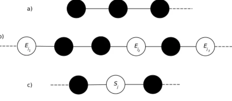
Assume thatGhas no isolated vertices. The reduction sendsGto an instanceφ(G) of TDS which will havem+n+ 1 colours: B (for black),Ei with 1≤i≤m(for the ith edge), andSj with 1≤j ≤n (for the jth vertex). The path has 9n+ 3 vertices altogether, starting with three black vertices of Figure 4(a), we call this tripletV0. Afterwards blocks of 6 and 3 vertices alternate, we call the latter V1, . . . , Vn, representing the vertices ofG. EachVj (other thanV0) is coloured as shown in Figure 4(c).
Assuming thatvj (1≤j≤n) is incident to the edgesej1,ej2, andej3, the two partsVj−1andVj are joined by a path representing these three incidences, and coloured as in Figure 4(b). Ifvj has degree less than 3, then the vertex in place ofEj3 is black; and ifd(vj) = 1, then alsoEj2 is black.
Figure 4: Gadgets for the reduction of Theorem 5.5
Letσ⊆V be an arbitrary solution to φ(G). First, we construct a solution σ0 fromσ with more structure, and with a measure at most that ofσ. For every j,σcontains the vertex coloured Sj. Let σ0 contain these as well. At least one of the first two vertices coloured B must also be in σ. Letσ0 contain the second vertex colouredB. Now, if anyVj (0≤j≤n) has a further (first or third) vertex which is an element ofσ, then we can replace it with its predecessor or successor, achieving that they dominate more vertices in the path. This modification does not lose any colour because the first and third vertices of anyVj are black, and B is already represented in σ∩V0.
Now we turn to the 6-element blocks connecting aVj−1 withVj. Since the third vertex ofVj−1 and the first vertex ofVj are surely not in the modifiedσ, which still dominates the path, it has to contain at least two vertices of the 6-element block. And if it contains only two, then those necessarily are the second and fifth, both being black. Should this be the case, we keep them inσ0. Otherwise, if the