The Czech Academy of Sciences, Institute of Geonics journal homepage: http://www.geonika.cz/mgr.html
doi: https://doi.org/10.2478/mgr-2020-0004
MORAVIAN GEOGRAPHICAL REPORTS
MORAVIAN GEOGRAPHICAL REPORTS
Illustrations related to the paper by R. Blaheta et al. (photo: T. Krejčí, E. Nováková (2×), Z. Říha) Fig. 5. Professor Eva Zažímalová, president of the Czech Academy of Sciences, presents Professor Bryn Greer-Wootten with the honorary medal
Fig. 6. Professor Bryn Greer-Wootten has his speech during the award ceremony Fig. 4. The Löw-Beer Villa in Brno, a place of the award ceremony Fig. 3. Members of the International Advisory Board of the MGR journal in front of the Institute of Geonics
Using local climate zones to compare remotely sensed surface temperatures in temperate cities
and hot desert cities
Cathy FRICKE
a, Rita PONGRÁCZ
b *, Tamás GÁL
a, Stevan SAVIĆ
c,János UNGER
aAbstract
Urban and rural thermal properties mainly depend on surface cover features as well as vegetation cover.
Surface classification using the local climate zone (LCZ) system provides an appropriate approach for distinguishing urban and rural areas, as well as comparing the surface urban heat island (SUHI) of climatically different regions. Our goal is to compare the SUHI effects of two Central European cities (Szeged, Hungary and Novi Sad, Serbia) with a temperate climate (Köppen-Geiger’s Cfa), and a city (Beer Sheva, Israel) with a hot desert (BWh) climate. LCZ classification is completed using WUDAPT (World Urban Database and Access Portal Tools) methodology and the thermal differences are analysed on the basis of the land surface temperature data of the MODIS (Moderate Resolution Imaging Spectroradiometer) sensor, derived on clear days over a four-year period. This intra-climate region comparison shows the difference between the SUHI effects of Szeged and Novi Sad in spring and autumn. As the pattern of NDVI (Normalised Difference Vegetation Index) indicates, the vegetation coverage of the surrounding rural areas is an important modifying factor of the diurnal SUHI effect, and can change the sign of the urban-rural thermal difference. According to the inter-climate comparison, the urban-rural thermal contrast is the strongest during daytime in summer with an opposite sign in each season.
Key words: satellite images, surface temperature, local climate zones, temperate and hot desert cities, Hungary, Serbia, Israel
Article history: Received 10 August 2019, Accepted 10 February 2020, Published 31 March 2020
a Department of Climatology and Landscape Ecology, University of Szeged, Szeged, Hungary
b Department of Meteorology, Eötvös Loránd University, Budapest, Hungary (*corresponding author: R. Pongrácz, e-mail: rita.pongracz@ttk.elte.hu)
c Climatology and Hydrology Research Centre, Faculty of Sciences, University of Novi Sad, Novi Sad, Serbia
1. Introduction
Urban areas substantially modify the radiative, thermal, moisture and aerodynamic conditions with more vegetation and less artificial surfaces on the local scale and mesoscale (Oke et al., 2017), creating a so-called urban climate different from the surrounding area. These modified features are also different within the city, depending on the characteristics of the built-up areas and anthropogenic activities (intra- urban differences). One of the most common phenomena associated with cities is the urban heat island (UHI) effect, which can be detected in near-surface air (Ta), as well as in surface temperature (Ts) (surface UHI, SUHI: e.g. Rasul et al., 2017). This can be easily quantified as the temperature difference between urban and rural areas, although the terminology of these areas is not straightforward in the literature (e.g. Stewart, 2007). In the case of Ts, several
remotely sensed land cover products (Imhoff et al., 2010;
Pongrácz et al., 2010; Zhou et al., 2013b; Mathew et al., 2018) and even night-time light data (Clinton and Gong, 2013; Fu and Weng, 2018) have been used to determine the boundary between urban and rural polygons.
2. Theoretical background
The concept of local climate zones (LCZs) has become a widely-used, universal framework, which is applicable for representing the lack of homogeneity of surface structures and land cover characteristics, even on the intra-urban scale, and therefore it can underlie the delineation of urban and rural areas. Its first formulation was released in Stewart (2009), and in its final form in Stewart and Oke (2012).
It consists of 10 built-up and 7 land cover classes. Originally,
this surface classification scheme was designed for the description of the surroundings of Ta measurement sites, but nowadays it has several applications. The first published study about an extension of LCZ beyond its primary functions, was in the mapping of zones in the urban area of a medium-sized Central European city (Novi Sad, Serbia), in order to recommend representative station sites for an urban climate monitoring network (Unger et al., 2011). The applied mapping process was relatively simple, as it was based on only the visual inspection of aerial images and the authors’
local knowledge.
Some time later, Bechtel and Daneke (2012), Bechtel et al. (2015) and Lelovics et al. (2014), developed more objective LCZ mapping methods; then, others followed them with the elaboration and comparison of different mapping approaches (e.g. Geletič and Lehnert, 2016;
Quan et al., 2017; Wang et al., 2018b; Hidalgo et al., 2019;
Mushore et al., 2019). Today, the LCZ-system is used worldwide, and the recent comparisons of thermal features in neighbourhoods with different built-up area characteristics, revealed definite Ta-differences between the zones; thus they confirmed the usefulness of the scheme (e.g. Stewart et al., 2014; Unger et al., 2015;
Leconte et al., 2015, 2017; Skarbit et al., 2017; Kotharkar and Bagade, 2018; Shi et al., 2018; Yang et al., 2018).
Besides these studies directed at Ta characteristics, the mapping of LCZs has expanded the application possibilities of the zones (Geletič et al., 2016). For instance, in recent years the scheme also provided a basis for some inter- LCZ thermal comparisons, using surface temperatures derived from remotely-sensed measurements. Some of these comparisons use airborne or high-resolution remote sensing data, but these are essentially case studies with small datasets. In comparison, Skarbit et al. (2015) applied high resolution Ts data acquired by an airborne small- format digital imaging system, measured on an August night in Szeged, Hungary. Bartesaghi Koc et al. (2018) used LiDAR-derived parameters to evaluate the quality of LCZ classifications by a comparison of mean values of Ts.
Nassar et al. (2016) investigated the LCZ–Ts relationship, applying Moderate Resolution Imaging Spectroradiometer (MODIS) 8-day composites from a year-long period, supplemented with nine Landsat scenes in Dubai (United Arab Emirates). Their analysis targetted the effects of different urban zones with varying structures, cover types and proximity to the ocean, urban cooling and heating in a city with dry desert climate. Wang et al. (2018a) also studied this relationship in arid cities in the south-western United States (Phoenix and Las Vegas), based on two night-time and two daytime ASTER (Advanced Spaceborne Thermal Emission and Reflection Radiometer) images from the warmer part of the year (May, August). They concluded that this type of analysis of LCZs provides valuable information about the distributions of land surface temperatures at the neighbourhood scale. Mushore et al. (2019) used cloud-free Landsat 8 imagery and WUDAPT methodology to monitor Ts patterns in Zimbabwe – on three cool days and three hot days. A study from the wet subtropical Yangtze River Delta (China) mega-region has to be mentioned: it acquired Ts from 13 Landsat and ASTER images (Cai et al., 2018). Their results also confirm that Ts is generally consistent with those LCZs showing higher Ts values in built-up LCZs.
Gémes et al. (2016) examined the seasonal development of urban Ts in the same study area using 7 Landsat thermal images, during a period of 30 years and 7 images
within a year. Also in Central Europe, Geletič et al. (2016) studied Prague and Brno (Czech Republic) using 8 Landsat and 8 ASTER thermal images, eight images for each city, which were obtained in the warmer months of the year.
Summarising their results, the variation of Ts is generally consistent with the LCZ classes as they have a higher temperature observed in built-up area classes. Recently, Geletič et al. (2019) performed an inter- and intra-zonal investigation of three Central-European cities (Prague, Brno and Novi Sad) and they also analysed the role of the vegetation in the Ts pattern. The results show that the character of the vegetation has well-marked effect on the intra-zonal seasonal variability of Ts.
Up to the present, most of the thorough longer-term investigations based on a continuous dataset have focused on the Ts-differences of urban-rural areas, defined by different subjective techniques, and they do not apply LCZ mapping for characterisation and separation in and around urban areas.
For instance, Zhou et al. (2013b) systematically analysed the daytime SUHI of European cities using MODIS-Aqua imagery between 2006 and 2011. They calculated the SUHI as the difference between the mean Ts of urban and rural clusters as defined by CORINE land cover data. They showed that the SUHI of many city clusters was higher in spring than in autumn. This result is considered a consequence of a phase shift between the astronomical and meteorological seasonality of Ts in the urban area and its surroundings.
According to further sensitivity simulations in London (Zhou et al., 2016), this hysteresis can be explained by the region- specific seasonal variation of solar radiation.
Peng et al. (2012) selected 419 large cities to quantify inter-city differences and explore the global drivers of SUHI.
They used MODIS-Aqua Ts data during the 2003–2008 period to report that cities with a more seasonal greening contrast between urban and suburban areas have a more pronounced seasonal SUHI effect. They also analysed the relationship between diurnal and nocturnal SUHI, and no correlation was found between them, which can be explained by the fact that driving mechanisms during the day are different from those at night.
Several Central European cities (i.e. Belgrade, Munich, Vienna, Milan, Warsaw, Zagreb and Budapest) were investigated by Pongrácz et al. (2010), between 2001 and 2003 using MODIS Ts and land cover products. According to the measurements in most of the examined cities, the nocturnal SUHI intensity was near-permanent (2–3 °C) between spring and autumn. The maximum intensity of SUHI occurred in daytime in summer, and the monthly mean intensity changed in a range from 1 °C to 6 °C. Tran et al. (2006) focused on eight Asian megacities that are located in both temperate and tropical climates. The most severe SUHI intensity (12 °C) was observed in Tokyo within a period of three years.
Zhou et al. (2013a) evaluated the diurnal variation of SUHI in Beijing on the basis of four typical 24-hour daily cycles in 2005, using MODIS data as well as in situ measurements.
In addition to the temporal cycle, they also analysed the spatial extension of the SUHI in Beijing.
From the research studies cited above, it can be concluded that there is a shortage of LCZ–Ts relationship investigations that are based on a large number of thermal images, enabling detailed diurnal and seasonal analysis.
In this paper we intend to reveal the urban-rural and intra- urban surface thermal reactions, and their differences (ΔTs) between Central European cities (Szeged, Hungary and Novi Sad, Serbia) with a warm and humid temperate climate
(Köppen type Cfa), as well as a city with a hot desert climate (Beer Sheva, Israel) (Köppen type BWh), based on a 4-year series of satellite data. Hence, the general aim is to depict the diurnal and seasonal evaluation of mean ΔTs values based on the cloud-free thermal pictures of MODIS in the period of 2014–2018.
Our specific objectives are to:
i. map LCZ patterns by city based on Landsat images;
ii. reveal the differences in the distribution of LCZs by climatic region;
iii. separate the ‘urban’ and ‘rural’ areas containing 1-km tiles according to the MODIS grid;
iv. determine the clearly distinguishable (representative) LCZ cells within the urban areas;
v. collect MODIS thermal images with clear conditions and separate them according to season (winter and summer), as well as night and day;
vi. compare the obtained mean seasonal and diurnal urban- rural Ts differences between the Cfa and BWh climatic regions (Szeged, Novi Sad vs. Beer Sheva); and
vii. compare the obtained mean seasonal and diurnal Ts differences of specific LCZs and rural areas between the Cfa and BWh climatic regions (Szeged, Novi Sad vs. Beer Sheva).
3. Data and methods
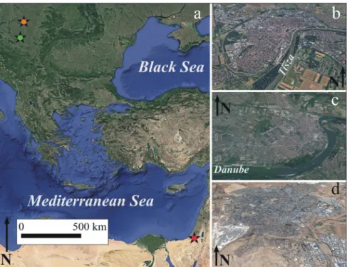
Figure 1 illustrates the locations of the studied cities and the general characteristics (aridity, vegetation) of their regions based on a colour Google Maps image.
Szeged (Hungary) and Novi Sad (Serbia) are located on the Great Hungarian (or Pannonian) Plain in Central Europe (see Fig. 1a). They have similar geographical and climatic environments: both of them can be found on mostly flat terrains and are in Köppen’s climatic region Cfa characterised by a warm and humid temperate climate, with a relatively warm summer and no distinguishable dry season (Beck et al., 2018). Szeged has a densely-built midrise core
of the city that becomes more open towards the suburban areas (Fig. 1b). The north-eastern part of the city consists of blocks of flats, while the suburbs are characterised by warehouses and detached houses with gardens. The neighbouring rural area is used for cultivating wheat, maize and other crops, but a few scattered trees are also found there (Skarbit et al., 2017). The central area of Novi Sad is densely built and wide avenues connect different areas of the city, which can be mainly characterised by midrise and low-rise built-up types (Fig. 1c). Warehouses and industrial zones are located in the northern suburban areas. The city surroundings are predominantly characterised by arable land, as well as dense and scattered tree areas (Unger et al., 2011).
Beer Sheva is the largest city in the Negev desert of southern Israel. In contrast to the previous two cities, it has a hot arid climate with Mediterranean influences (Köppen type BWh: Beck et al., 2018). It is one of the fastest growing cities in Israel; the development of its present cityscape has occurred only in the last century (Fig. 1d).
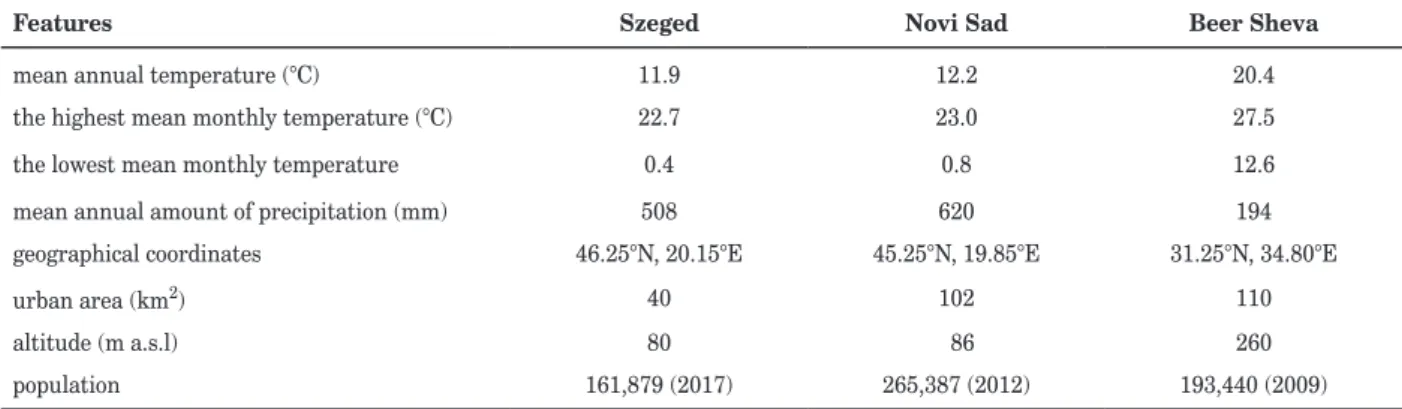
The historical city centre, built in the late Ottoman era, has been surrounded by several new urban neighbourhoods built in recent decades. The new part of Beer Sheva consists of 17 residential districts, as well as a university campus, hospitals, information technology and biotechnological centres. Its rural surroundings are dry and bare, occasionally with some vegetated patches. Table 1 summarises the main climatic and geographical features of the studied cities.
Considering that the mapping method of Bechtel et al.
(2015) uses open-access software and remotely sensed data, which has a homogeneous fine scale coverage, we applied this globally comprehensive classification method in this paper. This method is also applied in the worldwide WUDAPT (World Urban Database and Access Portal Tools) project (www.wudapt.org; Bechtel et al., 2019), as it provides a simple and objective workflow for LCZ mapping.
Two freely accessible software programs are required (i.e.
Google Earth and SAGA-GIS) to process all the 11 spectral bands of the Landsat 8 satellite imagery as input data. The multi-temporal, highest quality level (Level-1) Precision
Fig. 1: (a) Locations of the studied cities (stars: Szeged – orange; Novi Sad – green; Beer Sheva – red) and their aerial views: (b) Szeged, (c) Novi Sad and (d) Beer Sheva. Source: https://www.google.com/maps
Terrain data of the OLI (Operational Land Imager) and the TIRS (Thermal Infrared Sensor) instruments was retrieved from the Earth Explorer user interface of the U.S. Geological Survey. Cloud-free Landsat 8 images were selected for each city, which were taken in three different sections in the year (Szeged: 24.06.2017, 27.08.2017, 30.10.2017; Novi Sad: 04.03.2017, 24.06.2017, 30.10.2017;
Beer Sheva: 17.09.2017, 19.10.2017, 07.01.2018) to represent the intra-annual changes. Although the high resolution Landsat 8 images (30–100 m) are ideal for the mapping, we need to resample the images to a common resolution (100 m) in SAGA-GIS, which is acceptable for monitoring local patterns. Due to the annual course of surface properties, satellite images from different seasons are used for the LCZ mapping.
The first part of the process is to define the sample areas of the LCZ classes (training area polygons) and the region of interest (ROI) in Google Earth, called the training area (see Fig. 2). Each training area needs to be at least a 500 m × 500 m polygon with homogeneous structure, and the ROI must be a square-shaped polygon that covers the urban site, including the agglomeration and its surrounding natural environment. These delineated training area polygons and ROI are retained in a kml format file. In SAGA-GIS we perform the vector and raster processing using this kml file and Landsat 8 multispectral satellite images. A random forest classification algorithm performs the automated classification of Landsat images using the training polygons as learning areas within the ROI. If the classification does not take place properly, we have to improve the training areas and repeat the workflow. In the end, we perform a majority filtering that scans the neighbouring pixels within a given distance of a central pixel according to the size of the filter radius. If a particular LCZ class is in the majority in this examined field, all pixels are changed to that LCZ class.
In this paper the selected size of the radius was 3 pixels;
because this reduces noise, however, it does not perform unreasonable generalisation. The result of this workflow is a final LCZ map with reduced noise due to the filter.
To analyse the thermal properties of the urban area over the four-year period (2014–2018), we used derived Version 6 products (MOD11A1 and MYD11A1) from the measurements of the MODIS sensor, which can be found on the Terra and Aqua satellites. As parts of the American National Aeronautics and Space Administration’s (NASA) Earth Observing System, these solar-synchronous satellites (i.e. Terra and Aqua) carry out the tasks of providing data from different spheres of the Earth including the land surface, biosphere, hydrosphere, cryosphere and
atmosphere. The MODIS sensor measures radiation in 36 electromagnetic spectral bands with different spatial resolutions (250 m, 500 m, 1000 m) (NASA, 2006).
In this paper, we use Ts – derived from the raw MODIS radiation data – calculated from bands 3–7, 13 and 16–19 for retrieving emissivity, band 26 for cirrus cloud detection, and bands 20, 22, 23, 29, 31 and 32 for correction for atmospheric parameters (Wan and Dozier, 1996; Wan and Snyder, 1999).
Ts is retrieved by a generalised split-window algorithm. The quality of the data is improved by the optimisation of the algorithm coefficient to the viewing angle.
In addition, the method is less sensitive to uncertainty in emissivity over wide ranges of surface and atmospheric conditions. According to validations with in situ measurements, the MODIS Ts product accuracy is better than 1 °C over land (Wan et al., 2004; Wan and Dozier, 1996). Moreover, the quality assessment of Version 5 Ts by Wan (2008) and Wan and Li (2008) reported root mean square differences of less than 0.5 °C across 39 tested cases. The satellites can provide a total of four images per day for each city – hence, in this way we can consider two images for daytime and two images for night-time during 24 hours for the examined areas. The horizontal resolution of the thermal infrared measurements is 1 km, which is Tab. 1: Some climatic and geographical features of the studied cities
Sources: climate; 1986–2015 (Harris et al., 2014); geography; United Nations (2019)
Fig. 2: The processing scheme of LCZ mapping Source: authors, based on Bechtel et al., 2015
Features Szeged Novi Sad Beer Sheva
mean annual temperature (°C) 11.9 12.2 20.4
the highest mean monthly temperature (°C) 22.7 23.0 27.5
the lowest mean monthly temperature 0.4 0.8 12.6
mean annual amount of precipitation (mm) 508 620 194
geographical coordinates 46.25°N, 20.15°E 45.25°N, 19.85°E 31.25°N, 34.80°E
urban area (km2) 40 102 110
altitude (m a.s.l) 80 86 260
population 161,879 (2017) 265,387 (2012) 193,440 (2009)
appropriate in recognising the overall thermal pattern of the studied areas. More information about the specifications of the sensor is provided in Table 2.
Since an anticyclonic weather situation, with clear sky and low air movement, is the ideal weather condition to examine local-scale thermal features, we selected all clear days between the summer of 2014 and the spring of 2018. Considering the whole urban and rural area around the cities, we neglected all the days when any cloudy tile (cell) was detected (see Fig. 4 for their numbers by season and city).
One of our goals is to reveal the thermal differences between urban and rural areas. To complete a comprehensive study, it is especially important to define urban and rural areas as precisely as possible. In this study, we obtained the fractions of individual LCZ classes for each MODIS tile using the QGIS and based on these ratios we evaluated the building surface fraction of each cell. So, we consider ‘urban’
tiles that:
i. include at least 50% of built-up LCZ; and
ii. the cells form a coherent area (polygon) in order to neglect the effect of smaller, separated built-up patches near the suburban area; and
iii. to avoid the overspreading of the urban areas over the sparsely-built regions around the most urbanised areas, urban cells must be located within the administrative border of the city.
The specification of a representative rural area was a more complex challenge. In more detailed research, Pongrácz et al.
(2010) divided the urban and rural areas by the MODIS land cover product based on information about the elevation and radiation features of the surface. The urban area consisted of pixels with urban land cover within 15 km of the city centre, while the rural area is located in a radius belt of 15–25 km around the city centre. The pixels with hills were eliminated in the examined area.
Since we also require an area without any significant effects of built-up areas, water bodies or substantial topography, cells with a height difference above 200 m compared to the urban polygon or being covered by more than 1% of water, must be eliminated. Additionally, rural areas are defined as (i) mostly uninhabited, and (ii) being located at least 2 km
from the urban boundary. Hence, the rural areas form a belt of equal area around the urban area, similarly to previous works (e.g. Peng et al., 2012; Zhou et al., 2013b). The rural tiles (iii) must contain less than 1% of the total building surface fraction (TBSF) in order to avoid the effects of small towns and villages around delineated urban areas. As the building surface fraction (BSF) (Stewart and Oke, 2012) varies according to LCZ class, different ratios of LCZ class were allowed in rural tiles (Tab. 3). For example, when a tile contains LCZ 9, which has a minimum of 10% BSF, we eliminate this from the rural area, if the tile contains more than 10% of LCZ 9 due to it exceeding 1% TBSF of the entire tile. As an LCZ class shows higher BSF, we obviously take into account a smaller fraction of a tile.
Focusing on the thermal features of the individual urban LCZs, the investigation of representative areas of LCZ classes is required. For this purpose we selected MODIS tiles which have more than 55% coverage of a particular LCZ class. As a following step, mean Ts differences between the selected LCZs and rural areas were calculated for each cloud- free day and night, using the MOD11A1 and MYD11A1 images indicated above.
The satellite-derived Ts data series enable us to reveal the spatial and temporal features of the surface thermal features in the three target cities. First, we calculate the Ts mean values of the separated urban and rural areas for daytime (based on forenoon and afternoon MODIS images), and night-time (based on night and dawn images), in the case of each city. Then, we compute the mean diurnal and nocturnal Ts differences between urban and rural areas (SUHI intensity or ΔTs(u–r)). To retrieve the differences in thermal reactions caused by urban effects in the same and quite different climatic regions, the mean diurnal and nocturnal SUHI intensities between Szeged, Novi Sad (both Cfa) and Beer Sheva (BWh) were compared by season, and then the obtained differences are analysed and explained.
In addition we calculated the difference between the mean Ts of tiles with the same LCZ classes and the mean Ts of the rural area, as determined previously. The comparisons of the cities are presented in box-percentile plots (Esty and Banfield, 2003), which provide representative visualisations by showing the entire range and the distribution of the
Tab. 2: Technical features of the MODIS sensor Source: after Wan and Snyder (1999)
Tab. 3: Building surface fraction (BSF) of the built LCZ classes and the maximum possible value of the total building surface fraction (TBSF) of the cells considered as rural. Source: after Stewart and Oke, 2012
Sensor MODIS
satellite Terra Aqua
name of the product MOD11A1 MYD11A1
equatorial crossing times 10:30 a.m. (descending) 1:30 p.m. (ascending) acquisition times (UTC) 9–10 a.m. and 8–9 p.m. 2–3 a.m. and 12–13 p.m.
height ~705 km
LCZ classes BSF (%) Maximum TBSF (%)
compact midrise (2)/low-rise (3) 40–70 2.5
open-set midrise (5)/low-rise (6) 20–40 5
large low-rise (8) 30–50 3
sparsely built (9) 10–20 10
seasonal Ts differences. The boxes spread from minimum to maximum and the width contains detailed information about the distribution. The white lines – within the box – indicate the 25th percentile or lower quartile (near the bottom), the 50th percentile or median (in the middle) and the 75th percentile or upper quartile (near the top) value, therefore the area between the two quartiles represents half of all cases. The median has an advantage compared to the mean, namely, it is less affected by the extreme values. The black point – within the box – indicates the mean value of the Ts differences in each season. The numbers located near the horizontal axis of the diagram indicate the number of cases considered in the individual box above.
4. Results and discussion
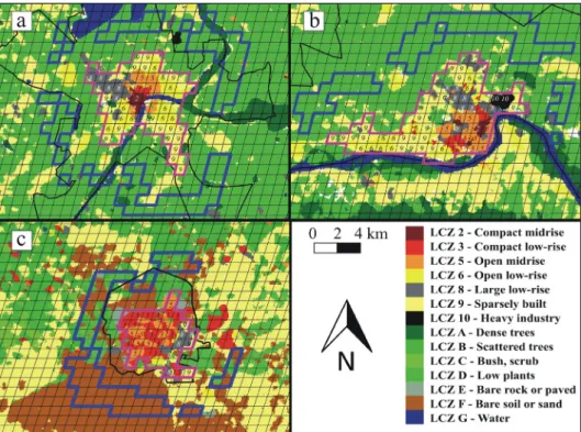
Figures 3a–3c present the obtained LCZ maps for Szeged, Novi Sad and Beer Sheva (hereinafter Sz, NS and BS), respectively. First of all, we can notice that three LCZ classes are absent in the urban areas: LCZ 1 (compact high- rise); LCZ 4 (open high-rise); and LCZ 7 (lightweight low- rise). In the case of NS and Sz, the administrative border – indicated with a black line – is located relatively distant from the city centre and encloses a large green area beside the built-up area (Figures 3a, b). In comparison to these cities, BS’s border is located nearby the mostly built-up core of the city (Fig. 3c). In addition, the administrative border separates broad, mostly sparsely-built (LCZ 9) regions from the central part of NS (to the south of the Danube) and BS (to the east of the city). Compact midrise classes (LCZ 2) are located in three different parts of the city in NS, LCZ 2 is situated in the city centre of Sz, whereas this zone is completely missing in BS. While the LCZ 3 (compact low- rise) and LCZ 5 (open midrise) classes are located north and south of the city centre in Sz, these LCZ classes are located near the city centre as well as in isolated patches at a greater distance from the centre both in NS and BS. The most
common classes around the central built-up area in Sz and NS are the open low-rise (LCZ 6) and sparsely built (LCZ 9) types, whereas these classes appear much less frequently within BS. There are also differences in the location of the large low-rise (LCZ 8) class, as the north-western part of Sz includes the LCZ 8 class, while this class is found in separated patches in NS (mostly in the northern half of the city) and in BS (in the southern part of the city). Heavy industry (LCZ 10) appears in both Central European cities and is associated with petroleum production and refining. It is located closer to the city centre and covers a larger area, however, in NS than in Sz.
The dominant land cover types around the two Central European cities are low plants with some dense and scattered trees (Figs. 3a, b). Some parts of the low plant areas temporarily change to bare soil within the year because of their agricultural use; thus, these two categories are merged into LCZ D. Since multiple satellite images from different dates are used to determine the different LCZs, the merging of the two zones simplifies the classification.
In contrast, around BS, beside the scattered trees and low plants, the other dominant land cover is sand because of the semi-arid environment (Fig. 3c). As a result for further investigations, Figure 3 also shows the delineated urban polygons and the separated rural tiles for each city determined by the selection procedure described above.
We selected tiles that are covered by particular LCZ classes over more than 55% of the tile area, and assigned them with the numbers of the majority LCZ class in each urban area.
These selected tiles were taken into consideration in the analysis of intra-urban and inter-urban thermal differences of the zones. Where there is no zonal number within the delineated urban area (Fig. 3), neither of the LCZ classes reached 55% coverage. Table 4 summarises the numbers of the selected urban tiles by zone and the numbers of the tiles in the rural areas assigned in and around the cities.
Fig. 3: LCZ maps shown on the MODIS grid covering the study areas: administrative city borders (black line);
delineated urban polygons (purple line); and rural (blue line) areas in and around (a) Szeged, (b) Novi Sad and (c) Beer Sheva (the selected LCZ tiles are marked by zone number)
Source: authors’ elaboration
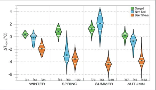
The seasonal urban-rural Ts differences (ΔTs(u–r)) in Szeged (Sz), Novi Sad (NS) and Beer Sheva (BS) that were detected on clear days in daytime are shown in Figure 4.
In Sz and in BS the largest absolute Ts difference values were detected in summer. In Sz the difference increases from winter to summer, then decreases in autumn. There is no substantial annual variation – the seasonal medians fluctuate between 0.3–1.3 °C – and the surface of the urban area is warmer than the rural area producing a recognisable SUHI effect in Sz. The medians of the ΔTs(u–r) have opposite sign throughout the year in BS, implying that the rural areas around BS are much warmer compared to the urban areas, therefore, the surface of the built-up area in BS acts as an urban cool island. This cooling effect of the delineated urban area is moderated (− 1.9 °C median) in winter and it increases throughout the year – ΔTs(u–r) reaches even − 6.5 °C in summer and autumn on certain days.
This opposite behaviour ensues from the fact that sand or dry bare soil is heated up more intensively by the stronger incoming solar radiation than in the Central European region, which is covered mostly with vegetation. In addition, in Central Europe the higher soil moisture content also helps to decrease Ts more effectively compared to BS.
Similar results were reported in cities surrounded by desert, such as Jeddah in Saudi-Arabia and Mosul in Iraq (Peng et al., 2012). Negative daytime SUHI intensity contributes to the oasis effect (Oke, 1987; Georgescu et al., 2011) caused by the residential and agricultural irrigation within the urban area. Georgescu et al. (2011) simulated this influence with the Weather Research and Forecasting
(WRF) regional climate model over Phoenix, Arizona. They concluded that besides the oasis effect, landscape and soil moisture conditions also explain the daytime cooling of urban areas. Observations from the United States also demonstrate the dependence of seasonal SUHI on biomes and environmental factors (Imhoff et al., 2010). The diurnal variation of thermal properties is discussed on the micro- scale by Zhan et al. (2012).
NS can be characterised by a high annual variation between the seasons. The sign of ΔTs(u–r) is mainly negative in all seasons except in summer, when a higher positive maximum of the median (2.1 °C) is observed than in Sz.
In summer, NS shows a larger fluctuation (from − 1.7 °C to 4.7 °C) in Ts differences, and the resulting SUHI effect of NS is mostly stronger (1–3.5 °C) compared to Sz (0.7–
1.7 °C). Moreover, a clear deviation was observed in spring:
the surface of the urban area was considerably cooler (by 2.9 °C on average and mostly 2.3–3.9 °C) in general than the rural area. In absolute terms, greater diurnal differences occur in spring (even 6 °C) than in summer (4.7 °C), when the urban area is heated by strong shortwave radiation causing a SUHI effect.
To reveal the reason for prominently negative ΔTs(u–r) values in NS, average spring NDVI (Normalised Difference Vegetation Index) values were calculated for each MODIS tile. The NDVI values shown in Figure 5 enable us to analyse the differences in the spatial distribution of the vegetation in the urban and the rural areas in both cities.
Figure 5a demonstrates that the rural area is characterised by higher NDVI values compared to the urban area in the Tab. 4: Numbers of the selected urban cells dominated by certain LCZs and rural cells by city
Source: authors’ elaboration
Fig. 4: Intra- (Cfa) and inter-climatic (Cfa vs. BWh) comparison of the diurnal urban-rural surface temperature differences (ΔTs(u-r)) by season (Szeged, Novi Sad vs. Beer Sheva, clear days, 01.06.2014–31.05.2018). Note: small numbers at the bottom of diagram = total numbers of selected satellite images by season in the studied cities Source: authors’ elaboration
City LCZ class (with more than 55% area coverage)
Rural
2 3 5 6 8 9 10
Szeged 2 1 3 10 6 18 0 84
Novi Sad 1 2 9 10 8 23 2 69
Beer Sheva 0 14 7 0 4 3 0 66
case of Sz. Figure 5b shows relatively low NDVI values in the rural area around NS, while the urban area has a similar pattern to Sz – the lowest mean NDVI values are detected in the most densely built-up areas (LCZs 2 and 3). In the surroundings of NS, the agricultural areas are mostly bare from autumn to spring (after the harvest and before the subsequent harvest), which leads to a rapid warm-up of the fields covered by dark soil in the morning, meanwhile the rural area around Sz is still covered by crops (as a result of the autumn sowing). Consequently, the rural areas of NS result in higher Ts values in spring than the rural areas of Sz.
According to the previous research of Savić et al. (2018) on the Ts -LCZ connection in the urban and the surrounding area of NS, during the vegetation period higher Ts values were detected in spring and autumn in the area covered with LCZ D compared to the built-up zones. The rural areas around NS and Sz are typically agricultural areas.
The arable lands around NS are covered mostly by dark chernozem soil (with low albedo), while the soil around Sz although of a similar texture, it additionally contains a certain fraction of sand, which makes it less dark, resulting in somewhat higher albedo.
In winter, there is no substantial thermal difference between Sz and NS as the medians of ΔTs(u-r) are around 0 °C in both cities, with the least variation among the seasons.
Finally, in autumn, the rural areas of NS are slightly warmer than the urban areas as the box extends between − 1.3 °C and 0.1 °C, meanwhile in Sz the distribution of ΔTs(u–r) is slightly more symmetrical with a small positive (0.3 °C) median value.
Similarly, different SUHI effects were detected in many European cities in spite of the same background temperature in spring and in autumn (Zhou et al., 2013b;
Zhou et al., 2016). This phenomenon is considered to be the result of different (astronomical and meteorological) seasonality in the urban and rural temperature, which can lead to differences in phenological phases.
The nocturnal urban-rural Ts differences (Fig. 6) clearly show less variability in the Central European cities, which is expected in an urban environment located in a moderate climate (e.g. Pongrácz et al., 2010). Generally, the urban areas are slightly warmer in the Central European cities than the corresponding rural areas. Meanwhile, in BS the mean seasonal ΔTs(u–r) values change between 0.2 °C and 0.5 °C throughout the year, which implies almost no thermal difference on average between the urban and rural areas; nevertheless, the rural area around BS is occasionally more than 2 °C warmer than the urban area in summer.
The mean seasonal ΔTs(u–r) of Sz reaches a maximum in summer, and then it decreases towards winter, while NS has a maximum in spring, which slightly exceeds the mean
Fig. 5: Distribution of mean spring NDVI in and around (a) Szeged and (b) Novi Sad (2014–2018) Source: authors’ elaboration
Fig. 6: Intra- (Cfa) and inter-climatic (Cfa vs. BWh) comparison of the nocturnal urban-rural surface temperature differences (ΔTs(u–r)) by season (Szeged, Novi Sad vs. Beer Sheva, clear nights, 01.06.2014–31.05.2018). Note: small numbers at the bottom of diagram = total number of selected satellite images by season in the studied cities
Source: authors’ elaboration
ΔTs(u–r) in summer. Furthermore, a clear difference can be recognised between the two Central European cities in spring: NS shows slightly higher Ts differences (mainly 1.4–1.7 °C) compared to Sz (mainly 0.8–1.4 °C). The medians of ΔTs(u–r) range between 0.6–1.6 °C, thus Ts values in both urban areas are typically higher than in the corresponding rural areas.
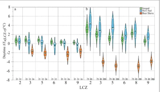
The diurnal mean LCZ-rural Ts differences compared for Sz, NS and BS measured on cloud-free days in two thermally extreme seasons (winter and summer), are presented in Figure 7. In winter the medians of the LCZs have no outstanding spatial variability considering the three cities together (Fig. 7a). Regarding the LCZ classes, there is no substantial difference between the two Central European cities. Sz and NS have similar medians: ΔTs(LCZ-r) of Sz fluctuates between 0.3 °C and 0.7 °C within the urban area, while the medians in NS are between 0 °C and 0.5 °C. In NS the diurnal ΔTs(LCZ-r) fluctuates over a larger range, and lower (occasionally negative) differences occur between the LCZs and the rural area compared to Sz.
For instance, the ΔTs(LCZ3-r) in Sz changes between − 0.6 °C and 1.7 °C, while the diurnal ΔTs values in NS are observed between − 2.3 °C and 2.5 °C during the examined period.
In BS, areas dominantly covered by LCZs 2 and 6 are not found, therefore they are absent from both Figures 7a and 7b. All of the LCZs are cooler in winter than the rural areas but there is no considerable discrepancy between them in their thermal reactions: the median of Ts difference was 1.6 °C for LCZs 3 and 9, meanwhile it was around 2 °C for LCZs 5 and 8.
In Sz and in NS the diurnal mean ΔTs(LCZ-r) values measured in summer generally fluctuate in a wider range than in winter (Fig. 7b). Due to the increased solar irradiation, the thermal differences between the LCZs are more conspicuous in the Central European cities. The strongest SUHI effect is detected in NS as the mean Ts differences of NS exceed the means of Sz considering each zone. The highest medians of the differences were observed between the most densely built-up class (LCZ 2) and the rural areas, both in Sz (3.3 °C) and in NS (4.5 °C). In Sz LCZ 2 is mainly warmer 2.2–4.4 °C than the surrounding
Fig. 7: Intra- (Cfa) and inter-climatic (Cfa vs. BWh) comparison of daytime mean LCZ-rural surface temperature differences (ΔTs(LCZ-r)) for (a) winter and (b) summer (Szeged, Novi Sad, Beer Sheva, clear days, 01.06.2014–
31.05.2018). Note: small numbers at the bottom of diagram = the total numbers of selected satellite images by season in the studied cities. Source: authors’ elaboration
rural area, while in NS this ΔTs changes mostly between 2.6 °C and 6.5 °C. Additionally, the difference reaches even 8 °C on certain days. In summer the medians of the diurnal ΔTs(LCZ-r) of Sz show a slight decrease moving from LCZ 2 (3.3 °C) to LCZ 9 (0.6 °C), except LCZ 8, where the median of ΔTs(LCZ-r) has a second maximum (2.2 °C). It shows consistency with the decreasing SUHI effect toward the border of the urban area as the Ts difference decreases proportionally with built-up area density. These results show good agreement with other studies (e.g. Thomas, et al., 2014; Mushore et al., 2019) suggesting that the most intense SUHI can be recorded in LCZ 2, while the weakest SUHI effect was detected in LCZ 9 in all seasons. In Sz and in NS, the sparsely-built (LCZ 9) zones show lower Ts compared to the rural areas, because of the higher ratio of vegetation, which has a cooling effect due to evaporation (Odindi et al., 2015; Stabler et al., 2015).
In BS all the zones are colder than the rural area in summer similarly to winter, but the absolute LCZ-rural ΔTs differences are greater in this season. The mean summer Ts values in LCZs 5 and 8 are around 5 °C lower than the rural values, which is beneficial for the population of the city. For LCZ 5 the largest absolute Ts difference is 7 °C, while for LCZ 8 the difference reaches 7.5 °C.
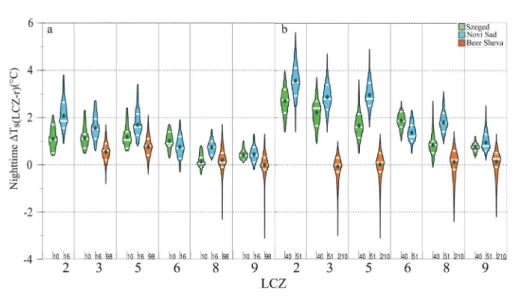
The nocturnal mean Ts differences between LCZs and the rural area that were measured on cloud-free days of winter and summer sorted by city, are shown in Figure 8. In winter (Fig. 8a), considering the Central European cities, the nocturnal Ts differences follow a similar pattern to the diurnal Ts-differences: the medians in Sz fluctuate mainly between 0.4 °C and 1.1 °C, and the medians in NS vary in the range of 0.4–1.9 °C with a slightly descending order from LCZ 2 to LCZ 9. In BS a weak SUHI was detected during winter nights: LCZs 3 and 5 are mainly 0.2–1 °C warmer than the rural area around BS. In LCZs 8 and 9 there are no considerable thermal differences compared to the rural area.
In summer (Fig. 8b) the nocturnal ΔTs(LCZ-r) values of Sz and NS fluctuate over a substantially smaller range compared to the daytime ranges, but nevertheless they follow similar patterns. In BS none of the zones are
considerably warmer than the rural surroundings, but some negative outliers can be found in each LCZ. In some extreme cases, Ts differences of around 3 °C occur (in LCZs 3 and 5).
The relatively high presence of the negative outliers shows that the rural area around BS is rather warmer compared to the LCZs at night as well (although it is clearly less warm than during the daytime).
5. Conclusions
In this study, the surface thermal features of three urban areas were compared, taking into account their specific climatic regions. Szeged and Novi Sad are located in a temperate climate, in Central Europe, whereas Beer Sheva is situated in the semi-arid climatic region of Israel. We used the clear-sky surface temperature data product of the MODIS sensor between the summer of 2014 and spring 2018.
To carry out comprehensive work, we performed LCZ mapping of the cities using the generally accepted WUDAPT methodology, and we delineated the urban and rural MODIS tiles according to different conditions in relation to the LCZ coverage. LCZ maps are able to illustrate the structure of the city that determines the thermal regimes. The seasonal urban-rural Ts differences were analysed and the results show that diurnal Ts differences are strongly affected by climatic conditions. Different urban effects were detected in the inter-climate comparison – the typical SUHI effect was recognised in Sz throughout the year in daytime, while the urban area showed a moderating/cooling effect in BS compared to the hot and semi-arid environment of the city.
As it can be expected, the most intense SUHI effect was observed in the central and industrial parts of the cities in a temperate climate in summer. Regional plans should focus on limiting the built-up area density or providing more open, green spaces in the problematic areas.
Additionally, differences were also seen in the intra-climate comparison of Sz and NS. The largest difference between the thermal features of the two cities with similar climatic conditions was detected in spring in daytime. According to the 4-year diurnal time series of the Ts differences, in spring and in autumn the rural area of NS warm up more intensively than the urban area, while in Szeged the SUHI effect was
Fig. 8: Intra- (Cfa) and inter-climatic (Cfa vs. BWh) comparison of nocturnal mean LCZ-rural surface temperature differences (ΔTs(LCZ-r)) for (a) winter and (b) summer (Szeged, Novi Sad, Beer Sheva, clear days, 01.06.2014–
31.05.2018). Note: small numbers at the bottom of diagram = the total numbers of selected satellite images by season in the studied cities. Source: authors’ elaboration
detected in accordance with the other seasons. Since the two cities are located in the same climate zone of the Köppen- Geiger system, the difference can be related to the vegetation coverage. The patterns of NDVI values show more abundant vegetation in the rural area of Sz than around NS in spring, therefore the phenomenon of the cooling island of NS could be the result of a quick warm up of the rural areas covered with thin vegetation.
Increasing the ratio of urban vegetation would be beneficial in both climatic regions, as (i) it helps to mitigate the urban-induced warming in a temperate climate, whereas (ii) vegetation improves the well-being of the habitants of cities surrounded by desert, so extending their vegetation cover is recommended. The results of this present study should be taken into account in developing environmental planning and mitigation strategies in urban areas in order to support sustainable local conditions.
In order to fully describe the relationship of Ts and vegetation, further research is required with more detailed remote sensing datasets. Namely, beside the temporal variation of the vegetation cover, soil moisture also plays a principle role in the thermal environment (e.g. Seneviratne et al., 2006). Future research should focus on this variable.
A better understanding of the spatial distributions of thermal properties and recognising the potentially problematic areas, will clearly contribute to more climate-sensitive urban planning for decision makers.
Acknowledgements
The MODIS data products were retrieved from the online Data Pool, courtesy of the NASA Land Processes Distributed Active Archive Center (LP DAAC), USGS/Earth Resources Observation and Science (EROS) Center, Sioux Falls, South Dakota, https://
lpdaac.usgs.gov/data_access/data_pool. Landsat data were retrieved from www.earthexplorer.usgs.com. This research has been partly supported by the National Research, Development and Innovation Office, Hungary (NKFI K-120346, K-120605, and K-129162), and the Ministry of Education, Science and Technological Development of the Republic of Serbia (Project No. 176020).
References:
BARTESHAGI KOC, C., OSMOND, P., PETERS, A., IRGER, M. (2018): Understanding land surface temperature differences of Local Climate Zones based on airborne remote sensing data. IEEE Journal of Selected Topics in Applied Earth Observations and Remote Sensing 11: 2724–2730.
BECHTEL, B., ALEXANDER, P. J., BÖHNER, J., CHING, J., CONRAD, O., FEDDEMA, F., MILLS, G., SEE, L., STEWART, I. (2015): Mapping Local Climate Zones for a worldwide database of the form and function of cities. ISPRS International Journal of Geo-Information, 4: 199–219.
BECHTEL, B., DANEKE, C. (2012): Classification of Local Climate Zones based on Multiple Earth observation data. IEEE Journal Selected Topics in Applied Earth Observation and Remote Sensing, 99: 1–5.
BECHTEL, B., ALEXANDER, P., BECK, C., BÖHNER, J., BROUSSE, O., CHING, J., DEMUZERE, M., FONTE, C., GÁL, T., HIDALGO, J., HOFFMANN, P., MIDDEL, A., MILLS, G., REN, C., SEE, L., SISMANIDIS, P., VERDONCK, M. L., XU, G., XU, Y. (2019): Generating WUDAPT Level 0 data – Current status of production and evaluation. Urban Climate, 27: 24–45.
BECK, H. E., ZIMMERMANN, N. E., MCVICAR, T. R., VERGOPOLAN, N., BERG, A., WOOD E. F. (2018):
Present and future Köppen-Geiger climate classification maps at 1-km resolution. Scientific Data, 5: 180–214.
CAI, M., REN, C., XU, Y., LAU, K. K-L., WANG, R. (2018):
Investigating the relationship between local climate zone and land surface temperature using an improved WUDAPT methodology – A case study of Yangtze River Delta, China. Urban Climate, 24: 485–502.
CLINTON, N., GONG, P. (2013): MODIS detected surface urban heat islands and sinks: global locations and controls. Remote Sensing of Environment, 134: 294–304.
ESTY, W. W., BANFIELD, J. (2003): The Box-Percentile Plot.
Journal of Statistical Software, 8(17): 1–14.
FU, P., WENG, Q. (2018): Variability in annual temperature cycle in the urban areas of the United States as revealed by MODIS imagery. ISPRS Journal of Photogrammetry and Remote Sensing, 146: 65–73.
GELETIČ, J., LEHNERT, M. (2016): A GIS-based delineation of local climate zones: The case of medium-sized Central European cities. Moravian Geographical Reports, 24(3): 2–12.
GELETIČ, J., LEHNERT, M., DOBROVOLNÝ, P. (2016):
Land surface temperature differences within Local Climate Zones, based on two Central European cities.
Remote Sensing, 8: 788.
GELETIČ, J., LEHNERT, M., SAVIĆ, S., MILOŠEVIĆ, D.
(2019): Inter-/intra-zonal seasonal variability of the surface urban heat island based on local climate zones in three central European cities. Building and Environment, 156: 21–32.
GÉMES, O., TOBAK, Z., VAN LEEUWEN, B. (2016): Satellite based analysis of surface urban heat island intensity.
Journal of Environmental Geography, 9: 23–30.
GEORGESCU, M., MOUSTAOUI, J. M., MAHALOV, J., DUDHIA, J. (2011): An alternative explanation of
the semiarid urban area “oasis effect”, Journal of Geophysical Research: Atmospheres, 116 (D24).
HARRIS, I., JONES, P. D., OSBORN, T. J., LISTER, D. H.
(2014): Updated high-resolution grids of monthly climatic observations – the CRU TS3.10 Dataset. International Journal of Climatology, 34: 623–642.
HIDALGO, J., DUMAS, G., MASSON, V., PETIT, G., BECHTEL, B., BOCHER, E., FOLEY, M., SCHOETTER, R., MILLS, G. (2019): Comparison between local climate zones maps derived from administrative datasets and satellite observations.
Urban Climate, 27: 64–89.
IMHOFF, M. L., ZHANG, P., WOLFE, R. E., BOUNOUA, L.
(2010): Remote sensing of the urban heat island effect across biomes in the continental USA. Remote Sensing of Environment, 114: 504–513.
KOTHARKAR, R., BAGADE, A. (2018): Evaluating urban heat island in the critical local climate zones of an Indian city. Landscape and Urban Planning, 169: 92–104.
LECONTE, F., BOUYER, J., CLAVERIE, R., PÉTRISSANS, M. (2015): Using Local Climate Zone scheme for UHI assessment: Evaluation of the method using mobile measurements. Building and Environment, 83: 39–49.
LECONTE, F., BOUYER, J., CLAVERIE, R., PÉTRISSANS, M. (2017): Analysis of nocturnal air temperature in districts using mobile measurements and a cooling indicator. Theoretical and Applied Climatology, 130: 365–376.
LELOVICS, E., UNGER, J., GÁL, T., GÁL, C. V. (2014):
Design of an urban monitoring network based on Local Climate Zone mapping and temperature pattern modelling. Climate Research, 60: 51–62.
MATHEW, A., KHANDELWAL, S., KAUL, N. (2018):
Analysis of diurnal surface temperature variations for the assessment of surface urban heat island effect over Indian cities. Energy and Buildings, 159: 271–295.
MUSHORE, T. D., DUBE, T., MANJOWE, M., GUMINDOGA, W., CHEMURA, A., ROUSTA, I., ODINDI, J., MUTANGA, O. (2018): Remotely sensed retrieval of Local Climate Zones and their linkages to land surface temperature in Harare metropolitan city, Zimbabwe. Urban Climate. 27: 259–271.
NASSAR, A. K., BLACKBURN, G. A., WHYATT, J. D (2016):
Dynamics and controls of urban heat sink and island phenomena in a desert city: Development of a local climate zone scheme using remotely-sensed inputs.
International Journal of Applied Earth Observation and Geoinformation, 51: 76–90.
ODINDI, J., BANGAMWABO, V., MUTANGA, O. (2015):
Assessing the value of urban green spaces in mitigating multi-seasonal urban heat using MODIS Land Surface Temperature (LST) and Landsat 8 data. International Journal of Environmental Research, 9: 9−18.
OKE, T. R. (1987): Boundary Layer Climates, 2nd edition.
London, Routledge.
OKE, T. R., MILLS, G., CHRISTEN, A., VOOGT, J. A. (2017):
Urban Climates. Cambridge, Cambridge University Press.
PENG, S., PIAO, S., CIAIS, P., FRIEDLINGSTEIN, P., OTTLE, C., BRÉON, F-M., NAN, H., ZHOU, L.,
MYNENI B. R. (2012): Surface urban heat island across 419 Global Big Cities. Environmental Science
& Technology, 46(2): 696−703.
PONGRÁCZ, R., BARTHOLY, J., DEZSŐ, Z. (2010):
Application of remotely sensed thermal information to urban climatology of Central European cities. Physics and Chemistry of the Earth, 35: 95–99.
QUAN, S. J., DUTT, F., WOODWORTH, E., YAMAGATA, Y., YANG, P. P-J. (2017): Local Climate Zone mapping for energy resilience: A fine-grained and 3D approach.
Energy Procedia, 105: 3777–3783.
RASUL, A., BALTZER, H., SMITH, C., REMEDIOS, J., ADAMU, B., SOBRINO, J. A., SRIVANIT, M., WENG, Q.
(2017): A review on remote sensing of urban heat and cool islands. Land, 6(2): 38.
SAVIĆ, S., GELETIČ, J., MILOŠEVIĆ, D., LEHNERT, M.
(2018): Analysis of land surface temperatures in the ‘local climate zones’ of Novi Sad (Serbia). Proceedings of the Cities and Climate Change Conference, Potsdam 2017.
Springer.
SENEVIRATNE, S. I., LÜTHI, D., LITSCHI, M., SCHAER, C. (2006): Land-atmosphere coupling and climate change in Europe. Nature, 443: 205–209.
SHI, Y., LAU, K. K-L., REN, C., NG, E. (2018): Evaluating the local climate zone classification in high-density heterogeneous urban environment using mobile measurement. Urban Climate, 25: 167–186.
SKARBIT, N., GÁL, T., UNGER, J. (2015): Airborne surface temperature differences of the different Local Climate Zones in the urban area of a medium sized city. Joint Urban Remote Sensing Event (JURSE), Lausanne, Switzerland, PID3445901.
SKARBIT, N., STEWART, I. D., UNGER, J., GÁL, T. (2017):
Employing an urban meteorological network to monitor air temperature conditions in the ‘local climate zones’ of Szeged, Hungary. International Journal of Climatology, 37/S1: 582–596.
STABLER, L. B., MARTIN, C. A., BRAZEL, A. J. (2005):
Microclimates in a desert city were related to land use and vegetation index. Urban Forestry Urban Greening, 3(3−4): 137−147.
STEWART, I. D. (2007): Landscape presentation and the urban-rural dichotomy in empirical urban heat island literature, 1950–2006. Acta Climatologica et Chorologica, 40–41: 111–121.
STEWART, I. D. (2009): Classifying urban climate field sites by “Local Climate Zones”. Urban Climate News, 34: 8–11.
STEWART, I. D., OKE, T. R. (2012): Local Climate Zones for urban temperature studies. Bulletin of American Meteorological Society, 93: 1879–1900.
STEWART, I. D., OKE, T. R., KRAYENHOFF, E. S. (2014):
Evaluation of the ‘local climate zone’ scheme using temperature observations and model simulations.
International Journal of Climatology, 34: 1062–1080.
THOMAS, G., SHERIN, A., ANSAR, S., ZACHARIAH, E.
(2014): Analysis of urban heat island in Kochi, India, using a modified local climate zone classification.
Procedia Environmental Sciences, 21: 3–13.
TRAN, H., UCHIHAMA, D., OCHI, S., YASUOKA, Y. (2006):
Assessment with satellite data of the urban heat island
effects in Asian mega cities. International Journal of Applied Earth Observation and Geoinformation, 8: 34–48.
UNGER, J., SAVIĆ, S., GÁL, T. (2011): Modelling of the annual mean urban heat island pattern for planning of representative urban climate station network. Advances in Meteorology, 2011: ID 398613.
UNGER, J., SAVIĆ, S., GÁL, T., MILOŠEVIĆ, D. (2014):
Urban climate and monitoring network system in Central European cities. Novi Sad – Szeged, University of Novi Sad/University of Szeged.
UNGER, J., GÁL, T., CSÉPE, Z., LELOVICS, E., GULYÁS, Á.
(2015): Development, data processing and preliminary results of an urban human comfort monitoring and information system. Időjárás, 119: 337–354.
UNITED NATIONS (2019): United Nations Demographic Yearbook 2017: Sixty-Eighth Issue, UN, New York.
WAN, Z. (2008): New refinements and validation of the MODIS land-surface temperature/emissivity products.
Remote Sensing of Environment, 112: 59–74.
WAN, Z., DOZIER, J. (1996): A generalized split-window algorithm for retrieving land-surface temperature from space. IEEE Transactions on Geoscience and Remote Sensing, 34: 892–905.
WAN, Z., LI, Z. L. (2008): Radiance-based validation of the V5 MODIS land-surface temperature product. International Journal of Remote Sensing, 29: 5373–5395.
WAN, Z., SNYDER, W. (1999): MODIS land-surface temperature algorithm theoretical basis document.
Institute for Computational Earth Systems Science, University of California, Santa Barbara.
WAN, Z., ZHANG, Y. L., ZHANG, Q. C., LI, Z. L. (2004):
Quality assessment and validation of MODIS global land surface temperature. International Journal of Remote Sensing, 25: 261–274.
WANG, C., MIDDEL, A., MYINT, S. W., KAPLAN, S., BRAZEL, A. J., LUKASCZYK, J. (2018a): Assessing local climate zones in arid cities: The case of Phoenix, Arizona and Las Vegas, Nevada. ISPRS Journal of Photogrammetry and Remote Sensing, 141: 59–71.
WANG, R., REN, C., XU, Y., LAU, K. K-L., SHI, Y. (2018b):
Mapping the local climate zones of urban areas by GIS- based and WUDAPT methods: A case study of Hong Kong. Urban Climate, 24: 567–575.
WUDAPT (World Urban Database and Access Portal Tools) [online]. [cit. 12.11.2019]. Available at: http://www.
wudapt.org
YANG, X., YAO, L., JIN, T., PENG, L. L. H., JIANG, Z., HU, Z., YE, Y. (2018): Assessing the thermal behavior of different local climate zones in the Nanjing metropolis, China. Building and Environment, 137: 171–184.
ZHAN, W., CHEN, Y., VOOGT, J., ZHOU, J., WANG, J., LIU, W., MA, W. (2012): Interpolating diurnal surface temperatures of an urban facet using sporadic thermal observations. Building and Environment, 57: 239–252.
ZHOU, J., CHEN, Y. C., ZHANG, X., ZHAN, W. (2013).
Modelling the diurnal variations of urban heat islands with multi-source satellite data. International Journal of Remote Sensing, 34(21): 7568–7588.
ZHOU, B., RYBSKI, D., KROPP, J. P. (2013): On the statistics of urban heat island intensity. Geophysical Research Letters, 40: 5486–5491.
ZHOU, B., LAUWAET, D., HOOYBERGHS, H., DE RIDDER, K., KROPP, J., RYBSKI, D. (2016): Assessing seasonality in the surface urban heat island of London.
Journal of Applied Meteorology and Climatology, 55: 493–505.
Please cite this article as:
FRICKE, C., PONGRÁCZ, R., GÁL, T., SAVIĆ, S., UNGER, J. (2020): Using local climate zones to compare remotely sensed surface temperatures in temperate cities and hot desert cities. Moravian Geographical Reports, 28(1): 48–60. Doi: https://doi.org/10.2478/
mgr-2020-0004