A possible general approach of the Apollonius problem with the help of
GeoGebra
László Budai
University of Debrecen budai0912@gmail.com
Submitted November 2, 2012 — Accepted November 28, 2012
Abstract
The Apollonius problem is one of the circle tangency problems that the eponymous Apollonius the “greatest Greek geometer” himself dealt with first and solved in general. Since then many people in many ways dealt with the problem. The new geometry is looking for ways to find simpler solutions for the problem differing from the draw up of elementary geometry. The current abstract shortly describes the frequent possible solution methods and more particularly deals with the three dimensional geometric solution methods as well as the practicability with the use in GeoGebra.
Keywords: Apollonius-problem, GeoGebra, cyclography MSC: M10, G10, G40
1. Introduction
Apollonius was born in Perga (Greece) around 262 BC. He conducted his mathe- matical studies in Alexandria in Euklides School where he also worked for a longer period of time. His works have not survived in originals; even one of them titled Konika on conic sections can be reached only in Arabic revision.
The original “Apollonius problem” is the following. Given three circles lying in the same plane, from these circles those need to be drawn up which are tangent with the three circles. If the radiuses of the given circles are reduced beyond all limits, then the circles are reduced to points or shrink into so called point circles. If
http://ami.ektf.hu
163
the radiuses of the given circles increase beyond all limits, then the circles become straight lines. Taking into consideration the this way generated degenerated cases we can conclude the following: from point, straight line and circle i.e. the number of combinations of the repetition of the three elements give all the possible problems.
Therefore we need to examine ten different tangency problems.
So, the amendment of the text for the problem can be the following: Those circles need to be drawn up that are points, straight lines and circles, on the same horizontal plane and from these they are tangent with three. In case if a circle is shrinking into a point the tangency means the fitting on the point.
Numbers of people ever since have dealt with solving these tangency problems such as: Viéte, Descartes, Newton, Lambert, Euler, Carnot, Gauss etc. The new geometry is seeking simpler ways for solutions, differing from elementary geometry draw ups, taking the problem out from plane and placing it into three dimensions, this way the draw up is done with the help of spheres or cones to perform the draw up.
2. Some more frequent methods for solving the prob- lem, brief
norder to perform the draw ups we can group the problems in such way that first we take the simple drawing up tasks and later from these take the hard draw ups and we can perform the more difficult draw ups or trace them back to simpler cases. We can use it for almost all solution methods which will be used.
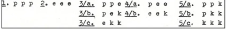
The grouping is as follows (Figure 1.):
Figure 1: The 10 problems built on each other
2.1. Elementary draw up
The 1st and the 2nd cases are the simplest cases and the draw ups can be car- ried out on the basis of elementary school knowledge: the perpendicular bisector segments defined by points represent the centre of the circle and in the 2nd case the geometrical place of the searchable centres of the circles are by the bisecting straight lines at the angle bisector and these are the intersections of the straight lines.
Solving case 3/a. can be summarized as follows: the geometrical place in case of searching for the centres of the circles to be identified by the straight line’s section bisector of two points specified by a straight line and the circles which is
providing solution for the problem has tangency points on the straight line and the perpendicular intersection drawn at the straight line by the point of contact on the straight line is giving the solution to the problem.
In case of 3/b. we can use a handy trick: let’s consider the problem solved, this way we can note some correlations of the geometrical place of the centres of the circles which are to be searched.
3/c. case is closely linked to the draw up done in case 3/b. Sub cases are obtained if we do the draw up by decreasing or increasing the radius (in this case the radius of the straight line is shifted with the given radius to a specific direction).
In short the solution for problem 4/a.: one point can be appointed anywhere after the draw up of the angel bisector identified by two straight lines, after this using similarity we arrive to the geometrical place of the centres of the circles searched.
The 4/b. problem can be traced back to problem 4/a.: we shrank the circles to points and shift the straight lines with the appropriate directionality.
Let’s consider the problem already solved during the solution of case 5/a., this way we arrive to the following: the geometrical place of the centres of the searched circles is the perpendicular intersection of the power points used as tangents to the circle and their contact points to the circle as well as the perpendicular bisector of the distance between the points.
We perform the 5/b. case draw up similarly, as the above techniques: the previous methods are used with the use of the similarity as far as the external and internal points.
The most obvious solution to case 5/c. is to trace it back to problem 5/b. The detailed elaboration with figures can be found among others in [1].
2.2. Problem solving with inversion
The inversion as a geometrical transformation is extremely suitable to solve such problems where circles, straight lines and their tangency are involved.
If the inversion is known as a transformation we can proceed as follows: the draw up of the circles contact points of the three circles can be simplified to the draw up of two given circles tangency points passing through one point of the drawn up circle (with decreasing the radius). Then when we select the specified point as a pole, the draw up is altered to the draw up of a straight line with tangency points with the circle as an inverse solution.
All possible solutions to the problem can be obtained by reducing or increasing the radius of the circles. Where straight lines are included also we need to apply the parallel shift of the straight lines instead of the increase/decrease of the radius.
This way we can carry out the solutions to all the problems (similar to those seen in the elementary draw up).
2.3. Hyperbola sections
The solution method originating from Adriaan van Roomen (1596) is based on the sections of two hyperboles. He simplified the problem with looking for tangent circles for two given circles. He concluded that the two tangential circles’ centres fall to that hyperbola, whose focal point coincides with the centres of the given circles. The centre of the searched circle and the difference of the distance between the centres of two given circles are independent from the radius of the tangential circles, those are permanent. Thus, the hyperbola’s sections belonging to the three circles in pairs are giving the centres of the searched circles.
It should be noted that Newton (1687) has further simplified the Roomen method: he has traced it back to the geometrical place of the centre of the searched tangency circles to the intersection of a point and a circle (trilateral problem).
2.4. Algebraic solution
Of course the Apollonius problem can be approached in an algebraic way. The base- line is the equation system which is arising from the coordinate-geometry equations of the given circles. With the help of the resultant we can reach the quadratic equa- tion system solutions, with the analysis of those the number of Apollonius problem solutions can be analysed (two real radicals, coinciding radicals, conjugated and complex solutions. . .).
2.5. Solution in three dimensions
If we place the problem from plane to three dimension then we arrive to a general solution of the problem with the help of spheres and cones. We will be dealing with this solution method in more detail later in chapter 3.
2.6. Gergonne type of solution
If three circles are given, draw up their exterior and interior similarity points.
Connect them with straight lines. We obtain four straight lines. Select one of them and determine the inverse of those points for each circle which are the closest to the circles. (Let’s take the pole of this straight line at the polar connection point for each circle). Then draw up the mutual power points which are determined by power lines of the three circles. This is the centre point of that circle which is perpendicularly intersecting all three circles. Let’s connect this with the previously given poles. These three lines are intersecting the three circles in two-two points these are going to be the tangency points. The three points out of the six needs to be chosen in a way as the lines have separated the circles. The point with a different characteristic needs to be chosen on that particular circle which is on the side of the straight line, then the other two with similar characteristics since they are positioned on the other side of the chosen straight line. The centre of the tangency circle can be drawn up from this point. Since there are four straight
lines, and we always arrive two tangency circles using this method we can always have all eight tangency circles.
2.7. The use of GeoGebra
The inclusion of a DGS into the geometry education is almost natural nowadays.
In case of the just examined problem it is especially true that it makes our job easier especially in the field of discussion. On a sheet of paper, we may choose any draw up methods; it is going to be difficult to follow the actual steps due to the lot of auxiliary lines. Not to mention if we would like to draw up all solutions on the paper and how we may want to add the 3 objects, so all the solutions may be visible on the paper.
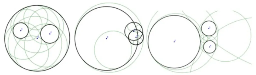
The following GeoGebra worksheet contains solutions for all 10 cases as a built in tool. (Figure 2):
Figure 2: Solutions of the Apollonius problems as a built in tool
Here you simply must select the particular case, after giving the input param- eters the tangency circles are going to be drawn. Parallel to the dynamic change of the given object it will dynamically change the placement of the tangent circles, giving an opportunity for a rapid discussion (Figure 3).
The before mentioned GeoGebra worksheet achieves the solutions for the first 9 problems with elementary draw ups. In case of the10th problem the solution is achieved by the help of hyperbola sections. Each macro tool can be opened from the menu, so with the function of replay the detailed draw up step sequence and the execution can be viewed.
Draw up executed by the way of inversion can be carried out similarly; the in- version has been built in as a tool into the GeoGebra worksheet for easier handling.
Figure 3: Given tangency circles in a given arrangement
3. Theoretical background of the three dimensional geometry solutions
One reasonable and advantageous problem solving mean to tackle plane geometrical draw ups is the index number portrayal (lative projection), which is one of the tool of cyclography. Cyclography was born with the help of the Apollonius type problem related search as simple and unified theoretical problem solution.
With the help of cyclographyc mapping lots of plane geometrical problems can be solved which would be very difficult to solve in the plane. So the problems are solve with the help of three dimensional objects, then the solutions are transformed back to the plane.
Let’s review briefly the cyclographyc mapping. Cyclography is not a type of linear mapping, where mutual definite relation is established between the points of three dimension and the plane directed circles. In cyclography in the plane of the drawing corresponds with the point of any of its circle which is in the centre of the circle on the perpendicular line of the plane of the drawing and is away from the centre of the circle with the distance of the radius. This way each circle corresponds with two points on the opposite side of the plane of the drawing. For clarity, we provide direction for the circle and it will be positive (counter clockwise) or negative (clockwise) in accordance with whether it is placed above the drawing of the plane of the corresponding point or below. The directed circles are called cycles after Laguerre. The image plane’s directed lines are called spreads. This can be interpreted as a cycle with an infinite radius. We need to handle the point as a cycle with zero radius. For every cycle and its corresponding point in three dimensions a 45◦ angular aperture size rotating cone can be fitted. We call this cone C cone (in case of a straight line it has a45◦ angular aperture to the image plane, can be treated also as a plane which fits to a given straight line).
Solving the Apollonius problem is getting simplified if we direct the circles and work with cycles this way. Then we search for cycles which are tangent to the three cycles. We know that the solution is given by the cyclographyc image of the mutual points of C cone belonging to the three cycles. The problem is thus lead back to the determination of the three C cone interpenetration effect.
Let us examine briefly the location of two different parallel rotating cones, their interpenetration effects as well as their common points. The interpenetration effect of the second-order cone is usually a fourth-order three dimensional curve. We also know that if two cones have two mutual tangential planes then the interpenetration effect will create two cone sections. In any case the parallel rotating cone has two mutual tangential planes which of course fit to the line which is connecting the vertex points of the cones. Therefore the interpenetration effect is always two cone sections. The question is where can we find these cone sections?
From depicting geometrical knowledge we can conclude the following: the three parallel rotating cones power plane defined in pairs intersect each other in one line in the power line of the three cones and the power line also fits to the plane of the interpenetration affect of the cones. It is obvious that it can intersect the cones only on the scone sections (up to two points if there are not indefinitely many points in common). Therefore the two thrust points are common points of all three cones. The daw up of the common points of the cones, which follows from the foregoing, can be simplified with the draw up of an intersection of a line and a cone (Figure 4.).
Figure 4: Common points of three cones
After this the general procedure for the actual draw up is the following:
1. We define the axis of the lineal cyclic congruence formed by the three cycles.
2. We draw up the power points of the three cycles (this will be the trace point of the straight multiplier).
3. We define the conjugate of the axis for some of the surface and with this we arrive to the three plane interpenetration affect of the intersection line.
4. With the given line status we draw a parallel through the power point, this way we arrive to the intersection line.
5. We thrust any of the cones with the intersection line. The cyclographyc images of the thrust points give the solution to the problem in case of directing the circles one way.
The original Apollonius problem has 8 solutions. By the way of cyclographic solutions it is as follows: We provide directions to the given three circles which will define by cycle one-one C cone. On these three cones we execute the prior draw up.
We may give directions to the three circles in total eight different ways, which may give in total 16 solutions. But considering the circles of solutions 8 solutions are to be considered. For example if the directing K1, K2, K3 circles by turns are +, +, - and -, -, + then the three dimensional elements used in the draw up (planes, cones etc.) are symmetrical to the plane of the drawing. The solution cycles are directed in an opposite way, but give identical circles. In (2) we can see detailed guidelines for all 10 cases.
4. The realization of three dimensional geometric so- lutions with GeoGebra
Why exactly GeoGebra?
On the internet there are two worksheets published, which solved the problem with cote projection mentioned in the previous chapter.
One is named Geometers sketch pad drawn up in DGS which is a paid service therefore a private citizen or an educational institution cannot access it free. The other was prepared in Carbi which can be viewed in a time and tool limited trial version. It only contains on case the problem of the three circles. In today’s Hungarian education systems it is a very important point of view (if not the most important) that the programs which are used would be free for the institution, teachers and students alike, due to the limited (financial) possibilities.
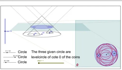
Taking into consideration the above mentioned shortcomings GeoGebra work- sheets have been prepared (Figure 5) which can be accessed at
http://geogebratube.com/student/m18934
URL and it is available and can be downloaded by anybody for free of charge.
Before discussing the possibilities of the program let’s have few words about the execution of the draw up. Since the steps of the draw up were rather general in the previous chapter, regarding the specific draw up executions in GeoGebra, for example looking at the three circles case we can simplify the draw ups by the following specifications. Let’s take the three given circles and consider it to one-one
Figure 5: Apollonius problem with cote projection in GeoGebra
cone’s level circle with the cote being 0. Let’s increase the radius of all three circles with the same interval; in this case in order to simplify the draw up let’s have the O2 cantered circle’s radius be the benchmark. Care must be taken during the draw up so the level circles would intersect each other in two-two points (in case we plan that the circles should be increasingly drifting away from each other, then it is better to take higher cote). With this interval we draw the level circles of the cones with 1-2 cotes, then we draw up the mutual power points of 1-2 level circles, which give us the 1-2 cote points of the power line’s of the three cones.
The further assignment is to draw up of the power line’s thrust point with some of the cones. In our case this is the cone which is fitting on the O2 level circle in order to draw simpler and less lines as just indicated before. The cote of the cone’s vertex is 1, so we just mete the divisor section of the line parallel to the power line.
The level line going through the 0 level point of the two straight lines out sects the base points of the two cone elements, the element also out sect from the searched power lines the thrust points, which are the geometrical places for the centres of the tangency circles.
Two cones belong to each circle and two planes fit on each straight line, which form symmetric pairs to the plane of the drawing.
The program contains two different views: one is the cones and their intersecting plane (that is parallel to the plane of the base circles); the other is perpendicularly showing from the top the actual status of the objects.
The plane can be moved with the slide called cote, this way it out sects level circles with different cote from the cones. The r1, r2 radiuses of the cones base circle are fitting to the base plane and can be set with a slide between 0 and 5.
The degenerated point circles arising from the level circles can be given in two different ways: If we set the radius to 0 or if the image plane is fitting exactly on
the vertex of the cone. We can arrive to a straight line if we move the image plane below the base plane. In theory the plane would need to move on the symmetrical oppositely directed cone, but since the radius cannot be increased infinitely (as in information technology infinite does not exist) therefore we simulate the circle with infinite radius this way. By the radius slides we can see the actual status of the objects in text display form.
The other view is to show the actual solutions; here we can see in an appropriate way the actual cotes of the level circles in accordance with the objects (point, circle, line). Here it should be mentioned that we have a very difficult job to do as far as drawing up techniques, if we want to arrive to a completely general and dynamic solution. Since it “costs a lot” that the objects can be located anywhere in relation to each other and the user can move them any way he/she pleases. The draw ups needed to be executed in several situations (for example, whether two pints are located inside or outside of the circle) or rather a relatively complex criteria system needed to be programmed to solve visibility issues.
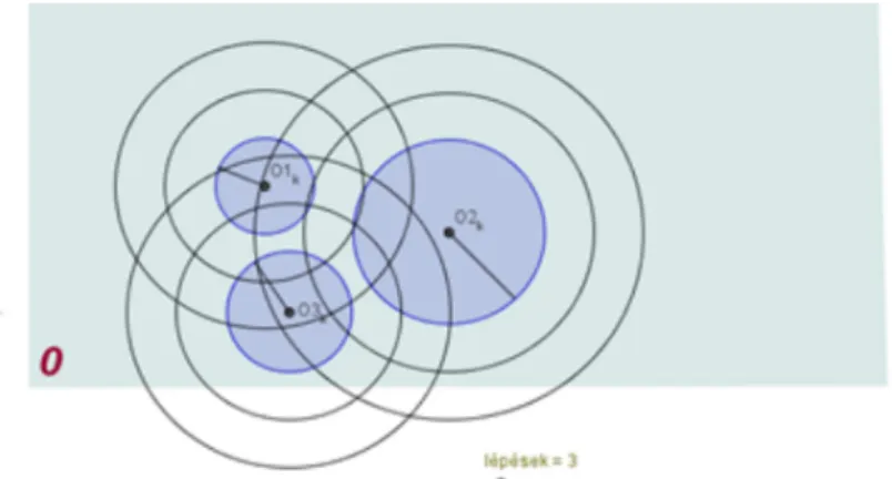
Since to show the solutions for each scenario is macro programmed (since Geo- Gebra could not not have handled safely the lots of objects and calculations on the worksheet) this way the built in function which plays back the draw up steps one by one cannot be used. Thus with the help of a slide called steps (if the conditions are right) we can follow the actual draw up steps (Figure 6.) shown with text descriptions and also with animation.
Figure 6: Presentation of the draw up steps
In my opinion the worksheet is suitable to present the Apollonius problem and to illustrate its general and elegant solutions as well as raise the demand for interest with reference to the topic.
References
[1] Maklári, J., Érintő körök szerkesztése sík-, és térmértani megoldással, illetve geomet- riai transzformációval,Tankönyvkiadó, 1963.
[2] Bácsó, S., Papp, I., Ciklográfiai példatár,Debreceni Egyetem, (jegyzet), 2006.
[3] Cranz, H., Das Apollonische berührungsproblem in stereographischer projektion, 1907.
[4] Hunyadi, J., Apollonius feladata a gömbfelületen,Bp., 1877.
[5] http://matematika.belvarbcs.hu/apollonius/index.htm (2012-10-31).
[6] Ripco Sipos, E., A geometria tanítása számítógép alkalmazásával, doktori (PhD) értekezés, 2011.
[7] http://salat.web.elte.hu/VIM/modules/apol_mod/apol_mod.htm (2012-10-31).
[8] http://mathworld.wolfram.com/ApolloniusProblem.html (2012-10-31).