Formal Languages and Automata Theory

(1)

Formal Languages and Automata Theory

Géza Horváth, Benedek Nagy

(2)

Formal Languages and Automata Theory

Géza Horváth, Benedek Nagy

(3)

Tartalom

Formal Languages and Automata Theory ... vi

Introduction ... vii

1. Elements of Formal Languages ... 1

1. 1.1. Basic Terms ... 1

2. 1.2. Formal Systems ... 2

3. 1.3. Generative Grammars ... 5

4. 1.4. Chomsky Hierarchy ... 6

2. Regular Languages and Finite Automata ... 12

1. 2.1. Regular Grammars ... 12

2. 2.2. Regular Expressions ... 16

3. 2.3. Finite Automata as Language Recognizers ... 19

3.1. 2.3.1. Synthesis and Analysis of Finite Automata ... 27

3.2. 2.3.2. The Word Problem ... 31

4. 2.4. Properties of Regular Languages ... 33

4.1. 2.4.1. Closure Properties ... 33

4.2. 2.4.2. Myhill-Nerode theorem ... 35

5. 2.5. Finite Transducers ... 36

5.1. 2.5.1. Mealy Automata ... 36

5.2. 2.5.2. Moore Automata ... 39

5.3. 2.5.3. Automata Mappings ... 42

3. Linear Languages ... 44

1. 3.1. Linear Grammars ... 44

2. 3.2. One-Turn Pushdown Automata ... 49

3. 3.3. Closure Properties ... 49

4. Context-free Languages ... 51

1. 4.1. Notation Techniques for Programming Languages ... 51

1.1. 4.1.1. Backus-Naur Form ... 51

1.2. 4.1.2. Syntax Diagram ... 51

2. 4.2. Chomsky Normal Form ... 52

3. 4.3. Pumping Lemma for Context-free Languages ... 56

4. 4.4. Closure Properties ... 57

5. 4.5. Parsing ... 58

5.1. 4.5.1. The CYK Algorithm ... 58

5.2. 4.5.2. The Earley Algorithm ... 60

5.2.1. Earley Algorithm ... 60

6. 4.6. Pushdown Automata ... 62

6.1. 4.6.1. Acceptance by Empty Stack ... 64

6.2. 4.6.2. Equivalence of PDAs and Context-free Grammars ... 67

6.3. 4.6.3. Deterministic PDA ... 68

6.4. 4.6.4. One-turn Pushdown Automata ... 68

5. Context-Sensitive Languages ... 71

1. 5.1. Context-Sensitive and Monotone Grammars ... 71

1.1. 5.1.1. Normal Forms ... 72

2. 5.2. Linear Bounded automata ... 77

3. 5.3. Properties of Context-Sensitive Languages ... 78

3.2. 5.3.2. About the Word Problem ... 80

6. Recursively Enumerable Languages and Turing Machines ... 82

1. 6.1. Recursive and Recursively Enumerable Languages ... 82

1.2. 6.1.2. Normal Forms ... 84

2. 6.2. Turing Machine, the Universal Language Acceptor ... 86

2.1. 6.2.1. Equivalent Definitions ... 88

3. 6.3. Turing Machine, the Universal Computing Device ... 89

4. 6.4. Linear Bounded Automata ... 91

7. Literature ... 94

(4)

Az ábrák listája

2.1. In derivations the rules with long right hand side are replaced by chains of shorter rules, resulting

binary derivation trees in the new grammar. ... 13

2.2. The graph of the automaton of Example 21. ... 21

2.3. The graph of the automaton of Exercise 19. ... 26

2.6. The graph of the automaton of Example 26. ... 28

2.7. The equivalence of the three types of descriptions (type-3 grammars, regular expressions and finite automata) of the regular languages. ... 30

2.11. The graph of the Mealy automaton of Example 30. ... 36

2.12. The graph of the Mealy automaton of Exercise 42. ... 39

3.1. In derivations the rules with long right hand side (left) are replaced by chains of shorter rules in two steps, causing a binary derivation tree in the resulting grammar (right). ... 46

4.1. Syntax diagram. ... 52

4.2. The triangular matrix M for the CYK algorithm. ... 59

4.3. The triangular matrix M for the CYK algorithm of the Example 45. ... 59

4.4. The triangular matrix M for the Earley algorithm. ... 60

4.5. The triangular matrix M for the Earley algorithm of the Example 46. ... 61

4.6. The graphical notation for the Example 47. ... 63

5.1. In derivations the rules with long right hand side are replaced by chains of shorter rules. ... 73

(5)

A táblázatok listája

4.1. Operations of the BNF metasyntax. ... 51

(6)

Formal Languages and Automata Theory

Géza Horváth, Benedek Nagy

University of Debrecen, 2014

Creative Commons NonCommercial-NoDerivs 3.0 (CC BY-NC-ND 3.0) A szerzők nevének feltüntetése mellett nem kereskedelmi céllal szabadon másolható, terjeszthető, megjelentethető és előadható, de nem módosítható.

Készült a TÁMOP-4.1.2.A/1-11/1-2011-0103 azonosítószámú „Gyires Béla Informatika Tárház” című projekt keretében.

(7)

Introduction

Formal Languages and Automata Theory are one of the most important base fields of (Theoretical) Computer Science. They are rooted in the middle of the last century, and these theories find important applications in other fields of Computer Science and Information Technology, such as, Compiler Technologies, at Operating Systems, ... Although most of the classical results are from the last century, there are some new developments connected to various fields.

The authors of this book have been teaching Formal Languages and Automata Theory for 20 years. This book gives an introduction to these fields. It contains the most essential parts of these theories with lots of examples and exercises. In the book, after discussing some of the most important basic definitions, we start from the smallest and simplest class of the Chomsky hierarchy. This class, the class of regular languages, is well known and has several applications; it is accepted by the class of finite automata. However there are some important languages that are not regular. Therefore we continue with the classes of linear and context-free languages.

These classes have also a wide range of applications, and they are accepted by various families of pushdown automata. Finally, the largest classes of the hierarchy, the families of context-sensitive and recursively enumerable languages are presented. These classes are accepted by various families of Turing machines. At the end of the book we give some further literature for those who want to study these fields more deeply and/or interested to newer developments.

The comments of the lector and some other colleagues are gratefully acknowledged.

Debrecen, 2014.

Géza Horváth and Benedek Nagy

(8)

(9)

1. fejezet - Elements of Formal Languages

Summary of the chapter: In this chapter, we discuss the basic expressions, notations, definitions and theorems of the scientific field of formal languages and automata theory. In the first part of this chapter, we introduce the alphabet, the word, the language and the operations over them. In the second part, we show general rewriting systems and a way to define algorithms by rewriting systems, namely Markov (normal) algorithms. In the third part, we describe a universal method to define a language by a generative grammar. Finally, in the last part of this chapter we show the Chomsky hierarchy: a classification of generative grammars are based on the form of their production rules, and the classification of formal languages are based on the classification of generative grammars generating them.

1. 1.1. Basic Terms

An alphabet is a finite nonempty set of symbols. We can use the union, the intersection and the relative complement set operations over the alphabet. The absolute complement operation can be used if a universe set is defined.

Example 1. Let the alphabet E be the English alphabet, the alphabet V contains the vowels, and the alphabet C is the set of the consonants. Then V∪C=E, V∩C=∅ and

A word is a finite sequence of symbols of the alphabet. The length of the word is the number of symbols it is composed of, with repetitions. Two words are equal if they have the same length and they have the same letter in each position. This might sound trivial, but let us see the following example:

Example 2. Let the alphabet V={1,2,+} and the words p=1+1, q=2. In this case 1+1≠ 2, i.e. p≠q, because these two words have different lengths, and also different letters in the first position.

There is a special operation on words called concatenation, this is the operation of joining two words end to end.

Example 3. Let the alphabet E be the English alphabet. Let the word p=railway, and the word q=station over the alphabet E. Then, the concatenation of p and q is p· q=railwaystation. The length of p is ∣ p∣ =7 and the length of q is ∣ q∣ =7, as well.

If there is no danger of confusion we can omit the dot from between the parameters of the concatenation operation. It is obvious that the equation ∣ pq∣ =∣ p∣ +∣ q∣ holds for all words p and q. There is a special word called an empty word, whose length is 0 and denoted by λ. The empty word is the identity element of the concatenation operation, λp=pλ=p holds for each word p over any alphabet. The word u is a prefix of the word p if there exists a word w such that p=uw, and the word w is a suffix of the word p if there exists a word u such that p=uw. The word v is a subword of word p if there exists words u,w such that p=uvw. The word u is a proper prefix of the word p, if it is a prefix of p, and the following properties hold: u≠λ and u≠p. The word w is a proper suffix of the word p, if it is a suffix of p, and w≠λ, w≠ p. The word v is a proper subword of the word p, if it is a subword of p, and v≠λ, v≠p. As you can see, both the prefixes and suffixes are subwords, and both the proper prefixes and proper suffixes are proper subwords, as well.

Example 4. Let the alphabet E be the English alphabet. Let the word p = railwaystation, and the words u=rail, v = way and w = station. In this example, the word u is a prefix, the word w is a suffix and the word v is a subword of the word p. However, the word uv is also a prefix of the word p, and it is a subword of the word p, as well. The word uvw is a suffix of the word p, but it is not a proper suffix.

We can use the exponentiation operation on a word in a classical way, as well. p⁰ = λ by definition, p¹ = p, and pⁱ

= p^i-1p, for each integer i ≥ 2. The union of pⁱ for each integer i ≥ 0 is denoted by p^*, and the union of pⁱ for each integer i ≥ 1 is denoted by p⁺. These operations are called Kleene star and Kleene plus operations. p^*=p⁺∪{λ} holds for each word p, and if p≠λ then p⁺=p^* \ {λ}. We can also use the Kleene star and Kleene plus operations on an alphabet. For an alphabet V we denote the set of all words over the alphabet by V^*, and the set of all words, but the empty word by V⁺.

(10)

A language over an alphabet is not necessarily a finite set of words, and it is usually denoted by L. For a given alphabet V the language L over V is L ⊆ V^*. We have a set again, so we can use the classical set operations, union, intersection, and the complement operation, if the operands are defined over the same alphabet. For the absolute complement operation we use V^* for universe, so We can also use the concatenation operation. The concatenation of the languages L1 and L2 contains all words pq where p ∈ L1 and q ∈ L2. The exponentiation operation is defined in a classical way, as well. L⁰={λ} by definition, L¹=L, and Lⁱ=L^i-1· L, for each integer i ≥ 2. The language L⁰ contains exactly one word, the empty word. The empty language does not contain any words, Le=∅, and L⁰ ≠ Le. We can also use the Kleene star and Kleene plus closure for languages.

so L^*=L⁺ if and only if λ ∈ L.

The algebraic approach to formal languages can be useful for readers who prefer the classical mathematical models. The free monoid on an alphabet V is the monoid whose elements are from V^*. From this point of view both operations, concatenation, (also called product) - which is not a commutative operation in this case -, and the union operation (also called addition), create a free monoid on set V, because these operations are associative, and they both have an identity element.

1. Associative:

• (L1 · L2) · L3 = L1 · (L2 · L3),

• (L1 ∪ L2) ∪ L3 = L1 ∪ (L2 ∪ L3), where L1, L2, L3 ⊆ V^*.

2. Identity element:

• L ⁰ · L1 = L1 · L⁰ = L1,

• Le ∪ L1 = L1 ∪ Le = L1, where L1 ⊆ V^*, L⁰= {λ}, Le = ∅.

The equation Le · L1 = L1 · Le = Le also holds for each L1 ⊆ V^*.

2. 1.2. Formal Systems

In this section, the definition of basic rewriting systems in general and a specific one, the Markov algorithm is presented.

Definition 1. A formal system (or rewriting system) is a pair W = ( V, P ), where V is an alphabet and P is a finite subset of the Cartesian product V^*× V^*. The elements of P are the (rewriting) rules or productions. If ( p, q ) ∈ P, then we usually write it in the form p → q. Let r, s ∈ V^*, and we say that s can be directly derived (or derived in one step) from r (formally: r ⇒ s) if there are words p, p', p'', q ∈ V^* such that r = p' pp'', s = p' qp'' and p → q ∈ P. The word s can be derived from r (formally: r ⇒^* s) if there is a sequence of words r0, r1, ..., rk ( k ≥ 1 ) such that r0 = r, rk = s and ri⇒ ri+1 holds for every 0 ≤ i < k. Moreover, we consider the relation r ⇒^* r for every word r ∈ V^*. (Actually, the relation ⇒^* is the reflexive and transitive closure of the relation ⇒.

A rewriting (or derivation) step can be understood as follows: the word s can be obtained from the word r in such a way that in s the right hand side q of a production of P is written instead of the left hand side p of the same production in r.

Example 5. Let W = ( V, P ) with V = { a, b, c, e, l, n, p, r, t } and P = { able → can, r → c, pp → b }. Then applerat ⇒ applecat ⇒ ablecat ⇒ cancat, and thus applerat ⇒^* cancat in the system W.

Now, we are going to present a special version of the rewriting systems that is deterministic, and was given by the Russian mathematician A. A. Markov as normal algorithms.

Definition 2. M = ( V, P, H ) is a Markov (normal) algorithm where

• V is a finite alphabet,

(11)

• P is a finite ordered set (list) of productions of the form V^* × V^*,

• H ⊆ P is the set of halting productions.

The execution of the algorithm on input w ∈ V^* is as follows:

1. Find the first production in P such that its left-hand-side p is a subword of w. Let this production be p → q. If there is no such a production, then step 5 applies.

2. Find the first (leftmost) occurrence of p in w (such that w = p'pp'' and p'p contains the subword p exactly once: as a suffix).

3. Replace this occurrence of p in w by the right hand side q of the production.

4. If p → q ∈ H, i.e., the applied production is a halting production, then the algorithm is terminated with the obtained word (string) as an output.

5. If there are no productions in P that can be applied (none of their left-hand-side is a subword of w), then the algorithm terminates and w is its output.

6. If a rewriting step is done with a non halting production, then the algorithm iterates (from step 1) for the newly obtained word as w.

We note here that rules of type λ → q also can be applied to insert word q to the beginning of the current (input) word.

The Markov algorithm may be terminated with an output, or may work forever (infinite loop).

Example 6. Let M = ({1,2,3 },{21→ 12, 31→ 13, 32→ 23},{}) be a Markov algorithm. Then, it is executed to the input 1321 as follows:

1321 ⇒ 1312 ⇒ 1132 ⇒ 1123.

Since there are no more applicable productions, it is terminated. Actually, it is ordering the elements of the input word in a non-decreasing way.

Example 7. Let

W=({a,b,c},{aa → bbb, ac→ bab, bc → a},{}).

Let us apply the algorithm W to the input

ababacbbaacaa.

As it can be seen in Animation 1 [3], the output is

ababbabbbbbabbb.

(For better understanding in the Animation the productions of the algorithm is numbered.)

Animation 1.

(12)

Exercise 1. Execute the Markov algorithm

M = ({ 1, + }, { 1 + → + 1, + + → +, + → λ } ,{ + → λ })

on the following input words:

• 1 + 1 + 1 + 1,

• 11 + 11 + 11,

• 111,

• 111 + 1 + 11.

Exercise 2. Execute the Markov algorithm M = ({1,×, a,b },

{ × 11 → a × 1, × 1 → a, 1a → a1b, ba → ab, b1 → 1b, a1 → a, ab → b, b → 1 } ,{ }) on the following input words:

• 1 × 1,

• 11 × 11,

• 111 × 1,

• 111 × 11.

The previous two exercises are examples for Markov algorithms that compute unary addition and unary multiplication, respectively.

It is important to know that this model of the algorithm is universal in the sense that every problem that can be solved in an algorithmic way can be solved by a Markov algorithm as well.

(13)

In the next section, other variations of the rewriting systems are shown: the generative grammars, which are particularly highlighted in this book. As we will see, the generative grammars use their productions in a nondeterministic way.

3. 1.3. Generative Grammars

The generative grammar is a universal method to define languages. It was introduced by Noam Chomsky in the 1950s. The formal definition of the generative grammar is the following:

Definition 3. The generative grammar (G) is the following quadruple:

G = ( N, T, S, P )

where

• N is the set of the nonterminal symbols, also called variables, (finite nonempty alphabet),

• T is the set of the terminal symbols or constants (finite nonempty alphabet),

• S is the start symbol, and

• P is the set of the production rules.

The following properties hold: N ∩ T = ∅ and S ∈ N.

Let us denote the union of the sets N and T by V ( V = N ∪ T). Then, the form of the production rules is V^*N V^*

→ V^*.

Informally, we have two disjoint alphabets, the first alphabet contains the so called start symbol, and we also have a set of productions. The productions have two sides, both sides are words over the joint alphabet, and the word on the left hand side must contain a nonterminal symbol. We have a special notation for the production rules. Let the word p be the left hand side of the rule, and the word q be the right hand side of the rule, then we use the p → q ∈ P expression.

Example 8. Let the generative grammar G be G = ( N, T, S, P ), where

N = {S,A}, T = {a,b}, andP = { S → bAbS,

bAb → bSab, A → λ, S → aa }.

In order to understand the operation of the generative grammar, we have to describe how we use the production rules to generate words. First of all, we should give the definition of the derivation.

Definition 4. Let G = ( N, T, S, P ) be a generative grammar, and let p and q be words over the joint alphabet V

= N ∪ T. We say that the word q can be derived in one step from the word p, if p can be written in a form p = uxw, q can be written in a form q = uyw, and x → y ∈ P. (Denoted by p ⇒ q.) The word q can be derived from the word p, if q = p or there are words r1, r2,..., rn such that r1 = p, rn = q and the word ri can be derived in one step from the word ri-1, for each 2 ≤ i ≤ n. (Denoted by p ⇒^* q.)

Now, that we have a formal definition of the derivation, let us see an example for deeper understanding.

Example 9. Let the generative grammar G be G = ( N, T, S, P ) , where

N = {S,A}, T = {0,1}, andP = { S → 1,

S → 1A,

(14)

A → AA, A → 0, A → 1 }.

Let the words p,t and q be p = A0S0, t = A01A0, and q = A0110. In this example, the word t can be derived from the word p in one step, (p → t), because p can be written in a form p = uxw, where u = A0, x = S, w = 0, and the word t can be written in a form t = uyw, where y = 1A, and S → 1A ∈ P.

The word q can be derived from the word p, (p ⇒^*q), because there exist words r1,r2 and r3 such that r1 = p, r2 = t, r3 = q and r1 ⇒ r2 and r2 ⇒ r3.

Now we have all the definitions to demonstrate how we can use the generative grammar to generate a language.

Definition 5. Let G = ( N, T, S, P ) be a generative grammar. The language generated by the grammar G is L(G)={p∣ p ∈ T^*, S ⇒^*p}.

The above definition claims that the language generated by the grammar G contains each word over the terminal alphabet which can be derived from the start symbol S.

Example 10. Let the generative grammar G be G = ( N, T, S, P ), where

N = {S,A}, T = {a,b}, andP = { S → bb,

S → ASA, A → a }.

In this example, the word bb can be derived from the start symbol S in one step, because S → bb ∈ P, so the word bb is in the generated language, bb ∈ L(G).

The word abba can be derived from the start symbol, because S ⇒ASA, ASA ⇒aSA, aSA ⇒ abbA, abbA → abba, so the word abba is also in the generated language, abba ∈ L(G).

The word bab can not be derived from the start symbol, so it is not in the generated language, bab ∉ L(G).

In this case, it is easy to determine the generated language, L(G) = {aⁱbbaⁱ∣ i ≥ 0}.

Exercise 3. Create a generative grammar G, which generates the language L = {a^*b⁺c^*}!

Exercise 4. Create a generative grammar G, which generates the language of all binary numbers!

4. 1.4. Chomsky Hierarchy

The Chomsky hierarchy was described first by Noam Chomsky in 1956. It classifies the generative grammars based on the forms of their production rules. The Chomsky hierarchy also classifies languages, based on the classes of generative grammars generating them. The formal definition is provided below.

Definition 6. (Chomsky hierarchy) Let G = ( N, T, S, P ) be a generative grammar.

• Type 0 or unrestricted grammars. Each generative grammar is unrestricted.

• Type 1 or context-sensitive grammars. G is called context-sensitive, if all of its production rules have a form p 1 Ap 2 → p1qp2,

or

S → λ,

(15)

where p 1 , p 2 ∈ V^*, A ∈ N and q ∈ V⁺. If S → λ ∈ P then S does not appear in the right hand side word of any other rule.

• Type 2 or context-free grammars. The grammar G is called context-free, if all of its productions have a form A → p,

where A ∈ N and p ∈ V^*.

• Type 3 or regular grammars. G is called regular, if all of its productions have a form A → r,

or

A → rB,

where A,B ∈ N and r ∈ T^*.

Example 11. Let the generative grammar G 0 be G

0 = ({S,X},{x,y},S,P) P = {

S → SXSy, XS → y, X → SXS, S → yxx }.

This grammar is unrestricted, because the second rule is not a context-sensitive rule.

1 = ({S,X},{x,y},S,P) P = {

S → SXSy, XSy → XyxXy, S → yXy, X → y }.

This grammar is context-sensitive, because each production rule has an appropriate form.

2 = ({S,X},{x,y},S,P) P = {

S → SyS, S → XX, S → yxy, X → ySy, X → λ }.

This grammar is context-free, because the left hand side of each production rule is a nonterminal symbol.

Example 14. Let the generative grammar G be

G = ({S,X},{x,y},S,P) P = {

S → xyS, S → X,

(16)

X → yxS, S → x, X → λ }.

This grammar is regular, because the left hand side of each production rule is a nonterminal, and the right hand side contains at most one nonterminal symbol, in last position.

Exercise 5. What is the type of the following grammars?

1. G = ({S,A},{0,1},S,P) P = {

S → 0101A, S → λ, A → 1S, A → 000 }.

2. G = ({S,A,B},{0,1},S,P) P = {

S → 0A01B, S → λ,

0A01 → 01A101, A → 0BB1, B → 1A1B, B → 0011, A → 1 }.

3. G = ({S,A,B},{0,1},S,P) P = {

S → 0ABS1, S → 10, 0AB → 01SAB, 1SA → 111, A → 0, B → 1 }.

4. G = ({S,A},{0,1},S,P) P = {

S → 00A, S → λ, A → λ, A → S1S }.

Definition 7. The language L is regular, if there exists a regular grammar G such that L = L (G).

The same kind of definitions are given for the context-free, context-sensitive, and recursively enumerable languages:

Definition 8. The language L is context-free, if there exists a context-free grammar G such that L = L (G).

Definition 9. The language L is context-sensitive, if there exists a context-sensitive grammar G such that L = L (G).

Definition 10. The language L is called recursively enumerable, if there exists an unrestricted grammar G such that L = L (G).

Although these are the most often described classes of the Chomsky hierarchy, there are also a number of subclasses which are worth investigating. For example, in chapter 3 we introduce the linear languages. A grammar is linear, if it is context-free, and the right hand side of its rules contain maximum one nonterminal symbol. The class of linear languages is a proper subset of the class of context-free languages, and it is a proper superset of the regular language class. Example 15. [9] shows a typical linear language and a typical linear grammar.

(17)

Example 15. Let L be the language of the palindromes over the alphabet T = {a,b}. (Palindromes are words that read the same backward or forward.) Language L is generated by the following linear grammar.

G = ({S},{a,b},S,P) P = {

S → aSa, S → bSb, S → a, S → b, S → λ }.

Language L is linear, because it can be generated by the linear grammar G.

Example 16. In Example 9 [5] we can see a context-free grammar, which is not linear, because the production A → AA is not a linear rule. However, this context-free grammar generates a regular language, because the same language can be generated by the following regular grammar.

G = ({S,A},{0,1},S,P, andP = { S → 1A,

A → 1A, A → 0A, A → λ }.

It is obvious that context-sensitive grammars are unrestricted as well, because each generative grammar is unrestricted. It is also obvious that regular grammars are context-free as well, because in regular grammars the left hand side of each rule is a nonterminal, which is the only condition to be satisfied for a grammar in order to be context-free.

Let us investigate the case of the context-free and context sensitive grammars.

Example 17. Let the grammar G be

G = ({S,A},{x,y},S,P) P = {

S → AxA, A → SyS, A → λ, S → λ }.

This grammar is context-free, because the left hand side of each rule contains one nonterminal. At the same time, this grammar is not context-sensitive, because

• the rule A → λ is not allowed in context-sensitive grammars,

• if S → λ ∈ P, then the rule A → SyS is not allowed.

This example shows that there are context-free grammars which are not context-sensitive. Although this statement holds for grammars, we can show that in the case of languages the Chomsky hierarchy is a real hierarchy, because each context-free language is context-sensitive as well. To prove this statement, let us consider the following theorem.

Theorem 1. For each context-free grammar G we can give context-free grammar G', which is context-sensitive as well, such that L (G) = L (G').

Proof. We give a constructive proof of this theorem. We are going to show the necessary steps to receive an equivalent context-sensitive grammar G' for a context-free grammar G = ( N, T, S, P ).

1. First, we have to collect each nonterminal symbol from which the empty word can be derived. To do this, let the set U (1) be U (1) = {A∣ A ∈ N, A → λ ∈ P}. Then let U (i) = U (i-1) ∪ {A∣ A → B1B2...Bn ∈ P, B1, B2,...,

(18)

Bn ∈ U (i-1)}. Finally, we have an integer i such that U (i) = U (i-1) = U which contains all of the nonterminal symbols from which the empty word can be derived.

2. Second, we are going to create a new set of rules. The right hand side of these rules should not contain the empty word. Let P' = (P ∪ P1)\{A→ λ∣ A ∈ N}. The set P1 contains production rules as well. B → p ∈ P1 if B → q ∈ P and we get p from q by removing some letters contained in set U.

3. Finally, if S ∉ U, then G' = ( N, T, S, P' ). If set U contains the start symbol, then the empty word can be derived from S, and λ∈ L (G). In this case, we have to add a new start symbol to the set of nonterminals, and we also have to add two new productions to the set P1, and G' = ( N ∪{S'}, T, S', P' ∪ {S' → λ, S' → S}), so G' generates the empty word, and it is context sensitive.

QED.

Example 18. Let the context-free grammar G be

G = ({S,A,B},{x,y},S,P) P = {

S → ASxB, S → AA, A → λ, B → SyA }.

Now, we create a context-sensitive generative grammar G', such that L (G') = L (G).

1. U (1) = {A}, U (2) = {A,S} = U.

2. P' = {

S → ASxB, S → SxB, S → AxB, S → xB, S → AA, S → A,

B → SyA, B → yA, B → Sy, B → y }.

3. G' = ({S,A,B,S'},{x,y},S',P' ∪{S' → λ, S' → S}).

Exercise 6. Create a context-sensitive generative grammar G', such that L (G') = L (G)!

G = ({S,A,B,C},{a,b},S,P) P = {

S → aAbB, S → aCCb, C → λ, A → C, B → ACC, A → aSb }.

Exercise 7. Create a context-sensitive generative grammar G', such that L (G') = L (G)!

G = ({S,X,Y},{0,1},S,P) P = {

S → λ, S → XXY, X → Y0Y1, Y → 1XS1, X → S00S }.

(19)

In the following chapters we are going to investigate the language classes of the Chomsky hierarchy. We will show algorithms to decide if a word is in a language generated by a generative grammar. We will learn methods which help to specify the position of a language in the Chomsky hierarchy, and we are going to investigate the closure properties of the different language classes.

We will introduce numerous kinds of automata. Some of them accept languages, and we can use them as an alternative language definition tool, however, some of them calculate output words from the input word, and we can see them as programmable computational tools. First of all, in the next chapter, we are going to deal with the most simple class of the Chomsky hierarchy, the class of regular languages.

(20)

2. fejezet - Regular Languages and Finite Automata

Summary of the chapter: In this chapter, we deal with the simplest languages of the Chomsky hierarchy, i.e., the regular languages. We show that they can be characterized by regular expressions. Another description of this class of languages can be given by finite automata: both the class of deterministic finite automata and the class of nondeterministic finite automata accept this class. The word problem (parsing) can be solved in real-time for this class by the deterministic finite automata. This class is closed under regular and under set-theoretical operations. This class also has a characterization in terms of analyzing the classes of possible continuations of the words (Myhill-Nerode theorem). We also present Mealy-type and Moore-type transducers: finite transducers are finite automata with output.

1. 2.1. Regular Grammars

In order to be comprehensive we present the definition of regular grammars here again.

Definition (Regular grammars). A grammar G=(N,T,S,P) is regular if each of its productions has one of the following forms: A → u, A → uB, where A,B∈ N, u∈ T^*. The languages that can be generated by regular grammars are the regular languages (they are also called type 3 languages of the Chomsky hierarchy).

Animation 2. [12] presents an example for a derivation in a regular grammar.

Animation 2.

We note here that the grammars and languages of the definition above are commonly referred to as right-linear grammars and languages, and regular grammars and languages are defined in a more restricted way:

Definition 12. (Alternative definition of regular grammars). A grammar G = ( N, T, S, P ) is regular if each of its productions has one of the following forms: A → a, A → aB, S → λ, where A,B ∈ N, a ∈ T. The languages that can be generated by these grammars are the regular languages.

(21)

Now we show that the two definitions are equivalent in the sense that they define the same class of languages.

Theorem 2. The language classes defined by our original definition and by the alternative definition coincide.

Proof. The proof consists of two parts: we need to show that languages generated by grammars of one definition can also be generated by grammars of the other definition.

It is clear the grammars satisfying the alternative definition satisfy our original definition at the same time, therefore, every language that can be generated by the grammars of the alternative definition can also be generated by grammars of the original definition.

Let us consider the other direction. Let a grammar G = ( N, T, S, P ) may contain rules of types A → u and A → uB (A,B ∈ N, u ∈ T^*). Then, we give a grammar G' = ( N', T, S', P' ) such that it may only contain rules of the forms A → a, A → aB, S' → λ (where A,B ∈ N', a ∈ T) and it generates the same language as G, i.e., L (G) = L (G').

First we obtain a grammar G'' such that L (G) = L (G'') and G'' = ( N'', T, S, P'' ) may contain only rules of the following forms: A → a, A → aB, A → B, A → λ (where A,B ∈ N'', a ∈ T). Let us check every rule in P: if it has one of the forms above, then we copy it to the set P'', else we will do the following:

• if the rule is of the form A → a1... ak for k > 1, where ai ∈ T, i ∈{1,...,k}, then let the new nonterminals X1,..., Xk-1 be introduced (new set for every rule) and added to the set N'' and instead of the actual rule the next set of rules is added to P'': A → a1X1, X1 → a2X2, ..., Xk-2 → ak-1Xk-1, Xk-1 → ak.

• if the rule is of the form A → a1... akB for k > 1, where ai ∈ T, i ∈ {1,...,k}, then let the new nonterminals X1,..., Xk-1 be introduced (new set for every rule) and put to the set N'', and instead of the actual rule the next set of rules is added to P'': A → a1X1, X1 → a2X2, ..., Xk-2 → ak-1Xk-1, Xk-1 → akB.

When every rule is analyzed (and possibly replaced by a set of rules) we have grammar G''. It is clear that the set of productions P'' of G'' may contain only rules of the forms A → a, A → aB, A → a, A → λ (where A,B ∈ N'', a∈ T), since we have copied only rules from P that have these forms, and all the rules that are added to the set of productions P'' by replacing a rule are of the forms A → aB, A → a (where A,B ∈ N'', a ∈ T). Moreover, exactly the same words can be derived in G'' and in G. The derivation graphs in the two grammars can be mapped in a bijective way. When a derivation step is applied in G with a rule A → a1... that is not in P'', then the rules must be used in G'' that are used to replace the rule A → a1...: applying the first added rule first A → a1X1, then there is only one rule that can be applied in G'', since there is only one rule added with X1 in its left hand side... therefore, one needs to apply all the rules of the chain that was used to replace the original rule A → a1....

Then, if there is a nonterminal B at the end of the rule A → a1..., then it is located at the end of the last applied rule of the chain, and thus the derivation can be continued in the same way in both grammars. The other way around, if we use a newly introduced rule in the derivation in G'', then we must use all the rules of the chain, and also we can use the original rule that was replaced by this chain of rules in the grammar G. In this way, there is a one-to-one correspondence in the completed derivations of the two grammars. (See Figure 2.1. for an example of replacing a long rule by a sequence of shorter rules.)

2.1. ábra - In derivations the rules with long right hand side are replaced by chains of shorter rules, resulting binary derivation trees in the new grammar.

Now we may have some rules in P'' that do not satisfy the alternative definition. The form of these rules can only be A → B and C → λ (where A,B,C ∈ N'', C ≠ S). The latter types of rules can be eliminated by the Empty- word lemma (see Theorem 1. [9]). Therefore, we can assume that we have a grammar G''' = ( N''', T, S', P''' ) such that L (G''') = L (G) and P''' may contain only rules of the forms A → aB, A → B, A → a, S' → λ (where A,B ∈ N''', a∈ T and in case S' → λ ∈ P''' the start symbol S' does not occur on the right hand side of any of the rules of P'''). Let us define the following sets of nonterminals:

• let U1 (A) = {A},

• let Ui+1 (A) = Ui (A) ∪ {B ∈ N'''∣ ∃ C ∈ Ui (A) such that C → B ∈ P'''}, for i > 1.

(22)

Since N''' is finite there is a minimal index k such that Uk(A) = Uk+1(A). Let U(A) denote the set Uk(A) with the above property. In this way, U(A) contains exactly those nonterminals that can be derived from A by using rules only of the form B → C (where B,C ∈ N'''). We need to replace the parts A ⇒^*B → r of the derivations in G''' by a direct derivation step in our new grammar, therefore, let G' = ( N''', T, S', P' ), where P' = {A → r∣ ∃ B ∈ N''' such that B → r ∈ P''', r ∉ N''' and B ∈ U(A)}. Then G' fulfills the alternative definition, moreover, it generates the same language as G''' and G.

QED.

Further we will call a grammar a regular grammar in normal form if it satisfies our alternative definitions. In these grammars the structures of the rules are more restricted: if we do not derive the empty word, then we can use only rules that have exactly one terminal in their right hand side.

Example 19. Let

G = ({S,A,B},{0,1,2},S,

{ S → 010B, A → B, A → 2021, B → 2A, B → S, B → λ }).

Give a grammar that is equivalent to G and is in normal form.

Solution:

Let us exclude first the rules that contain more than one terminal symbols. Such rules are S → 010B and A → 2021. Let us substitute them by the sets

{S → 0X1, X1 → 1X2, X2 → 0B}

and

{A → 2X3, X3 → 0X4, X4 → 2X5, X5 → 1}

of rules, respectively, where the newly introduced nonterminals are {X1, X2} and {X3, X4, X5}, respectively. The obtained grammar is

G'' = ({S, A, B, X1, X2, X3, X4, X5},{0,1,2},S, { S → 0X1,

X1 → 1X2, X2 → 0B, A → B, A → 2X3, X3 → 0X4, X4 → 2X5, X5 → 1, B → 2A, B → S, B → λ ).

Now, by applying the Empty-word lemma, we can exclude rule B → λ (the empty word can be derived from the nonterminals B and A in our example) and by doing so we obtain grammar

G''' = ({S, A, B, X1, X2, X3, X4, X5}, {0,1,2}, S, { S → 0X1,

X1 → 1X2,

(23)

X2 → 0B, X2 → 0, A → B, A → 2X3, X3 → 0X4, X4 → 2X5, X5 → 1, B → 2A, B → 2, B → S }).

Now we are excluding the chain rules A → B, B → S. To do this step, first, we obtain the following sets:

U 0 (S) = {S} U 0 (A) = {A} U 0 (B) = {B}

U 1 (S) = {S} = U(S)

^U¹ (A) = {A,B} U 1 (B) = {B,S}

U 2 (A) = {A,B,S} U 2 (B) = {B,S} =

U(B) U 3 (A) = {A,B,S} =

U(A)

Actually for those nonterminals that are not appearing in chain rules these sets are the trivial sets, e.g., U (X1) = U0 (X1) = {X1}. Thus, finally, we obtain grammar

G' = ({S, A, B, X1, X2, X3, X4, X5}, {0,1,2}, S, { S → 0X1,

A → 0X1, B → 0X1, X1 → 1X2, X2 → 0B, X2 → 0, A → 2X3, X3 → 0X4, X4 → 2X5, X5 → 1, B → 2A, A → 2A, B → 2, A → 2 }).

Since our transformations preserve the generated language, every obtained grammar (G'', G''' and also G') is equivalent to G. Moreover, G' is in normal form. Thus the problem is solved.

Exercise 8. Let

G = ({S, A, B, C},{a,b},S,

{ S → abA, S → A, A → B, B → abab, B → aA, B → aaC, B → λ, C → aaS }).

Exercise 9. Let

G = ({S, A, B, C},{a,b,c},S,

(24)

{ S → A, S → B, A → aaB, B → A, B → acS, B → C, C → c, C → λ }).

Exercise 10. Let

G = ({S, A, B, C, D},{a,b,c},S,

{ S → aA, S → bB, A → B, B → A, B → ccccC, B → acbcB, C → caacA, C → cba }).

Exercise 11. Let

G = ({S, A, B, C, D},{1,2,3,4},S,

{ S → 11A, S → 12B, A → B, B → C, B → 14, B → 4431, C → 3D, D → 233C }).

2. 2.2. Regular Expressions

In this section, we will describe the regular languages in another way. First, we define the syntax and the semantics of regular expressions, and then we show that they describe the same class of languages as the class that can be generated by regular grammars.

Definition 13. (Regular expressions). Let T be an alphabet and V = T ∪ {∅, λ, +, ·, ^*,(,)} be defined as its extension, such that T ∩ {∅, λ, +, ·, ^*,(,)} = ∅. Then, we define the regular expressions over T as expressions over the alphabet V in an inductive way:

• Base of the induction:

• ∅ is a (basic) regular expression,

• λ is a (basic) regular expression,

• every a ∈ T is a (basic) regular expression;

• Induction steps

(25)

• if p and r are regular expressions, then (p+r) is also a regular expression,

• if p and r are regular expressions, then (p · r) is also a regular expression (we usually eliminate the sign · and write (pr) instead (p · r)),

• if r is a regular expression, then r^* is also a regular expression.

Further, every regular expression can be obtained from the basic regular expressions using finite number of induction steps.

Definition 14 (Languages described by regular expressions). Let T be an alphabet. Then, we define languages described by the regular expressions over the alphabet T following their inductive definition.

• Basic languages:

• ∅ refers to the empty language {},

• λ refers to the language {λ},

• for every a ∈ T, the expression refers to the language {a};

• Induction steps:

• if p and r refer to the languages Lp and Lr, respectively, then the regular expressions (p+r) refers to the language Lp∪ Lr,

• if p and r refer to the languages Lp and Lr, respectively, then the regular expressions (p · r) or (pr) refers to the language Lp · Lr,

• if r refers to a language Lr then r^* refers to the language Lr*.

The language operations used in the above definition are the regular operations:

• the addition (+) is the union of two languages,

• the product is the concatenation of two languages, and

• the reflexive and transitive closure of concatenation is the (Kleene-star) iteration of languages.

Two regular expressions are equivalent if they describe the same language. Here are some examples:

(p+r) ≡ (r+p) (commutativity of union)

((p+r)+q) ≡ (p+(r+q)) (associativity of union)

(r+∅) ≡ r (additive zero element,

unit element for union)

((pr)q) ≡ (p(rq) (associativity of

concatenation)

(rλ) ≡ (λr) ≡ r (unit element for

concatenation)

((p+r)q) ≡ ((pq)+(rq)) (left distributivity)

(p(r+q)) ≡ ((pr)+(pq)) (right distributivity)

(r∅) ≡ ∅ (zero element for

concatenation)

λ ^* ≡ λ (iteration of the unit

element)

∅ ^* ≡ λ (iteration of the zero

element)

(rr^*) ≡ (r^*r) (positive iteration)

(26)

Actually, the values of the last equivalence are frequently used, and they are denoted by r⁺, i.e., r⁺ ≡ rr^* by definition. This type of iteration which does not allow for 0 times iteration, i.e., only positive numbers of iterations are allowed, is usually called Kleene-plus iteration.

With the use of the above equivalences we can write most of the regular expressions in a shorter form: some of the brackets can be eliminated without causing any ambiguity in the language described. The elimination of the brackets is usually based on the associativity (both for the union and for the concatenation). Some further brackets can be eliminated by fixing a precedence order among the regular operations: the unary operation (Kleene-)star is the strongest, then the concatenation (the product), and (as usual) the union (the addition) is the weakest.

We have regular grammars to generate languages and regular expressions to describe languages, but these concepts are not independent. First we will prove one direction of the equivalence between them.

Theorem 3. Every language described by a regular expression can be generated by a regular grammar.

Proof. The proof goes by induction based on the definition of regular expressions. Let r be a basic regular expression, then

• if r is ∅, then the empty language can be generated by the regular grammar (S, A, T, S, {A → a});

• if r is λ, then the language {λ} can be generated by the regular grammar (S, T, S, {S → λ});

• if r is a for a terminal a ∈ T, then the language {a} is generated by the regular grammar (S, T, S, {S → a}).

If r is not a basic regular expression then the following cases may occur:

• r is (p+q) with some regular expressions p,q such that the regular grammars Gp = (Np, T, Sp, Pp) and Gq = (Nq, T, Sq, Pq) generate the languages described by expression p and q, respectively, where Np ∩ Nq = ∅ (this can be done by renaming nonterminals of a grammar without affecting the generated language). Then let

G = (Np ∪ Nq ∪ {S}, T, S, Pp ∪ Pq ∪ {S → Sp, S→ Sq}),

where S ∉ Np ∪ Nq is a new symbol. It can be seen that G generates the language described by expression r.

• r is (p · q) with some regular expressions p,q such that the regular grammars Gp = (Np, T, Sp, Pp) and Gq = (Nq, T, Sq, Pq) generate the languages described by expression p and q, respectively, where Np ∩ Nq = ∅. Then let

G = (Np ∪ Nq,T, Sp, Pq ∪ {A → uB∣ A → uB ∈ Pp, A,B ∈ Np, u ∈ T^*} ∪ {A → uSq∣ A → u

∈ Pp, A ∈ Np, u ∈ T^*}).

It can be shown that G generates the language described by expression r.

• r is a regular expression of the form q^* for a regular expression q. Further let Gq = (Nq, T, Sq, Pq) be a regular grammar that generates the language described by expression q. Then, let

G = (Nq ∪ {S},T,S, Pq ∪ {S → λ, S → Sq} ∪ {A → uSq∣ A → u ∈ Pq, A ∈ Nq, u ∈ T^*}), where S ∉ Nq. It can be shown that G generates the language described by expression r.

Since every regular expression built by finitely many applications of the induction step, for any regular expression one can construct a regular grammar such that the grammar generates the language described by the expression.

QED.

(27)

When we want to have a grammar that generates the language given by a regular expression, the process can be faster, if we know that every singleton, i.e., language containing only one word, can easily be obtained by a grammar having only one nonterminal (the start symbol) and only one production that allows to generate the given word in one step.

Example 20. Let r = (cbb)^*(ab+ba) be a regular expression (that describes a language over the alphabet {a,b,c}). Give a regular grammar that generates this language.

Solution:

Let us build up r from its subexpressions. According to the above observation, the language {cbb} can be generated by the grammar

Gcbb =({Scbb},{a,b,c},Scbb,{Scbb → cbb}).

Now, let us use our induction step to obtain the grammar G ( cbb )^* that generates the language (cbb)^*: then G ( cbb )^* = ({Scbb, S(cbb)^*},{a,b,c},S(cbb)^*,

{Scbb → ccb, S(cbb)^* → λ, S(cbb)^* → Scbb, S(cbb) → cbb S(cbb)}).

The languages {ab} and {ba} can be generated by grammars

Gab = ({Sab},{a,b,c},Sab,{Sab → ab}) and

Gab = ({Sba},{a,b,c},Sba,{Sba → ba}),

respectively. Their union, ab+ba, then is generated by the grammar

Gab+ba = ({Sab,Sba,Sab+ba},{a,b,c},Sab+ba,

{Sab → ab, Sba → ba, Sab+ba → Sab, Sab+ba → Sba}) according to our induction step.

Finally, we need the concatenation of the previous expressions (cbb)^* and (ab+ba), and it is generated by the grammar

G ( cbb ^*)( ab+ba ) = ({Scbb, S(cbb)^*,Sab,Sba,Sab+ba}, {a,b,c}, S(cbb)^*, {Scbb → cbbSab+ba, S(cbb)^* → Sab+ba, S(cbb)^* → Scbb, S(cbb)^* → cbb S(cbb)^*, Sab → ab, Sba → ba, Sab+ba → Sab, Sab+ba → Sba})

due to our induction step. The problem is solved.

Exercise 12. Give a regular expression that describes the language containing exactly those words that contain three consecutive a's over the alphabet {a,b}.

Exercise 13. Give a regular expression that describes the language containing exactly those words that do not contain two consecutive a's (over the alphabet {a,b}).

Exercise 14. Give a regular grammar that generates the language 0^*(1+22)(2^*+00).

Exercise 15. Give a regular grammar that generates the language 0+1(1+0)^*.

Exercise 16. Give a regular grammar that generates the language (a+bb(b+(cc)^*))^*(ababa+c^*).

3. 2.3. Finite Automata as Language Recognizers

(28)

In this section we first define several variations of the finite automata distinguished by the properties of the transition function.

Definition 15 (Finite automata). Let A = ( Q, T, q0, δ, F ). It is a finite automaton (recognizer), where Q is the finite set of (inner) states, T is the input (or tape) alphabet, q0 ∈ Q is the initial state, F ⊆ Q is the set of final (or accepting) states and δ is the transition function as follows.

• δ : Q × (T ∪ {λ}) → 2^Q (for nondeterministic finite automata with allowed λ-transitions);

• δ : Q × T → 2^Q (for nondeterministic finite automata without λ-transitions);

• δ : Q × T → Q (for deterministic finite automata, λ can be partially defined);

• δ : Q × T → Q (for completely defined deterministic finite automata (it is not allowed that δ is partial function, it must be completely defined).

One can observe, that the second variation is a special case of the first one (not having λ-transitions). The third variation is a special case of the second one having sets with at most one element as images of the transition function, while the fourth case is more specific allowing sets exactly with one element.

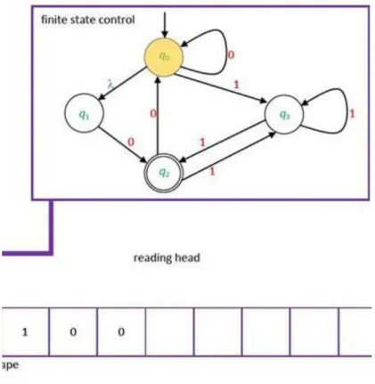
One can imagine a finite automaton as a machine equipped with an input tape. The machine works on a discrete time scale. At every point of time the machine is in one of its states, then it reads the next letter on the tape (the letter under the reading head), or maybe nothing (in the first variations), and then, according to the transition function (depending on the actual state and the letter being read, if any) it goes to a/the next state. It may happen in some variations that there is no transition defined for the actual state and letter, then the machine gets stuck and cannot continue its run.

There are two widely used ways to present automata: by Cayley tables or by graphs. When an automaton is given by a Cayley table, then the 0th line and the 0th column of the table are reserved for the states and for the alphabet, respectively (and it is marked in the 0th element of the 0th row). In some cases it is more convenient to put the states in the 0th row, while in some cases it is a better choice to put the alphabet there. We will look at both possibilities. The initial state should be the first among the states (it is advisable to mark it by a → sign also). The final states should also be marked, they should be circled. The transition function is written into the table: the elements of the set δ(q,a) are written (if any) in the field of the column and row marked by the state q and by the letter a. In the case when λ-transitions are also allowed, then the 0th row or the column (that contains the symbols of the alphabet) should be extended by the empty word (λ) also. Then λ-transitions can also be indicated in the table.

Automata can also be defined in a graphical way: let the vertices (nodes, that are drawn as circles in this case) of a graph represent the states of the automaton (we may write the names of the states into the circles). The initial state is marked by an arrow going to it not from a node. The accepting states are marked by double circles. The labeled arcs (edges) of the graph represent the transitions of the automaton. If p ∈ δ (q,a) for some p,q ∈ Q, a ∈ T ∪ {λ}, then there is an edge from the circle representing state q to the circle representing state p and this edge is labeled by a. (Note that our graph concept is wider here than the usual digraph concept, since it allows multiple edges connecting two states, in most cases these multiple edges are drawn as normal edges having more than 1 labels.)

In this way, implicitly, the alphabet is also given by the graph (only those letters are used in the automaton which appear as labels on the edges).

In order to provide even more clarification, we present an example. We describe the same nondeterministic automaton both by a table and by a graph.

Example 21. Let an automaton be defined by the following Cayley table:

T Q → q0 q 1 ⊂q2⊃ ⊂q3⊃

a q 1 q 1 q 2, q3 -

b q 0 q 0 - q 3

c q 0 q 2 - q 1,q2,q3