Parallel approach of algorithms
Herendi, Tamás
Nagy, Benedek
Parallel approach of algorithms
írta Herendi, Tamás és Nagy, Benedek Szerzői jog © 2014 Typotex Kiadó
Kivonat
Summary: Nowadays the parallelization of various computations becomes more and more important. In this book the theoretical models of parallel computing are presented. Problems that can be solved and problems that cannot be solved in these models are described. The parallel extensions of the traditional computing models, formal languages and automata are presented, as well as properties and semi-automatic verifications and generations of parallel programs. The concepts of theory of parallel algorithms and their complexity measures are introduced by the help of the (parallel) Super Turing-machine. The parallel extensions of context-free grammars, such as L-systems, CD and PC grammar systems; multihead automata (including various Watson- Crick automata), traces and trace languages are described. The theory and applications of Petri nets are presented by their basic concepts, special and extended models. From the practical, programming point of view, parallelization of (sequential) programs is investigated based on discovering of dependencies.
Copyright: Dr. Tamás Herendi, Dr. Benedek Nagy, University of Debrecen Creative Commons NonCommercial-NoDerivs 3.0 (CC BY-NC-ND 3.0)
This work can be reproduced, circulated, published and performed for non-commercial purposes without restriction by indicating the author's name, but it cannot be modified.
Reviewer: Iván Szabolcs ISBN 978 963 279 338 2
Prepared under the editorship of Typotex Kiadó Responsible manager: Zsuzsa Votisky
Made within the framework of the project Nr. TÁMOP-4.1.2/A/1-11/1-2011-0063, entitled „Sokprocesszoros rendszerek a mérnöki gyakorlatban”.
Tartalom
Introduction ... viii
1. Methods for analysis of algorithms ... 1
1.1. Mathematical background ... 1
1.1.1.1.1. The growth order of functions ... 1
1.1.1.1.2. Complexity concepts ... 7
1.2. Parallel computing models ... 10
1.2.1.2.1. Simulation ... 19
1.2.1.2.2. Complexity classes ... 22
3. Questions and problems ... 23
4. Literature ... 23
2. Parallel grammar models ... 25
2.1. An overview: Generative grammars, Chomsky-hierarchy ... 25
2.2. Indian, Russian and bounded parallel grammars ... 27
2.2.2.2.1. Indian parallel grammars ... 27
2.2.2.2.2. Russian parallel grammars ... 28
2.2.2.2.3. Grammars with bounded parallelism ... 29
2.2.2.2.3.2.2.3.1. k-parallel grammars ... 29
2.2.2.2.3.2.2.3.2. Scattered context grammars ... 30
2.2.2.2.3.2.2.3.3. Generalised parallel grammars ... 31
2.2.4. Questions and exercises ... 32
2.2.5. Literature ... 33
2.3. Lindenmayer-systems ... 33
2.3.2.3.1. 0L and D0L-system ... 33
2.3.2.3.2. Extended (E0L and ED0L) systems ... 38
2.3.2.3.3. Other variants ... 40
2.3.2.3.3.2.3.3.1. L-systems with finite sets of axiom (F0L) ... 40
2.3.2.3.3.2.3.3.2. Adult languages ... 41
2.3.2.3.4. Tabled systems ... 41
2.3.2.3.5. L-systems with interactions (IL) ... 44
2.3.2.3.6. Further remarks ... 45
2.3.7. Questions and exercises ... 47
2.3.8. Literature ... 48
2.4. CD and PC grammar systems ... 49
2.4.2.4.1. Cooperating Distributed (CD) grammar systems ... 49
2.4.2.4.1.2.4.1.1. Fairness of CD systems ... 52
2.4.2.4.1.2.4.1.2. Hybrid CD systems ... 52
2.4.2.4.2. Parallel Communicating (PC) grammar systems ... 53
2.4.2.4.2.2.4.2.1. PC systems communicating by commands ... 56
2.4.3. Questions and exercises ... 58
2.4.4. Literature ... 59
3. Parallel automata models ... 61
3.1. Recall: the traditional (sequential) finite state automata ... 61
3.2. Multihead automata ... 61
3.2.3.2.1. Watson-Crick finite automata ... 61
3.2.3.2.1.3.2.1.1. 5'→3' WK automata ... 63
3.2.3.2.2. m-head automata ... 65
3.2.3. Questions and exercises ... 69
3.2.4. Literature ... 70
3.3. P automata ... 70
3.3.1. Questions and exercises ... 73
3.3.2. Literature ... 74
3.4. Cellular automata ... 74
3.4.3.4.1. One-dimensional two-state cellular automata - Wolfram's results ... 77
3.4.3.4.2. Pattern growth ... 80
3.4.3.4.3. Conway's game of life ... 81
3.4.3.4.4. Other variations ... 85
3.4.5. Questions and exercises ... 86
3.4.6. Literature ... 87
4. Traces and trace languages ... 88
4.1. Commutations and traces ... 88
4.1.4.1.1. Commutations ... 88
4.1.4.1.2. Trace languages ... 93
2. Questions and exercises ... 98
3. Literature ... 99
5. Petri nets ... 101
5.1. Introduction ... 101
5.2. Binary Petri nets ... 101
5.3. Place-transition nets ... 109
5.3.5.3.1. Reduction techniques ... 116
5.3.5.3.2. Special place-transition nets ... 119
5.3.5.3.2.5.3.2.1. Marked graph model ... 119
5.3.5.3.2.5.3.2.2. Free-choice nets ... 119
5.4. Further Petri net models ... 121
5.4.5.4.1. Coloured Petri nets ... 121
5.4.5.4.2. Inhibitor arcs in Petri nets ... 121
5.4.5.4.3. Timed Petri nets ... 122
5.4.5.4.4. Priority Petri nets ... 122
5.4.5.4.5. Other variations of Petri nets ... 122
5.4.5.4.5.5.4.5.1. Reset nets ... 122
5.4.5.4.5.5.4.5.2. Transfer nets ... 122
5.4.5.4.5.5.4.5.3. Dual nets ... 122
5.4.5.4.5.5.4.5.4. Hierarchy nets ... 123
5.4.5.4.5.5.4.5.5. Stochastic, continuous, hybrid, fuzzy and OO Petri nets ... 124
5.4.5.5. Petri net languages ... 124
5. Questions and exercises ... 124
6. Literature ... 125
6. Parallel programs ... 127
6.1. Elementary parallel algorithms ... 127
6.1.6.1.1. Merge sort ... 130
6.1.6.1.2. Batcher’s even-odd sort ... 131
6.1.6.1.3. Full comparison matrix sort ... 132
6.2. Parallelization of sequential programs ... 133
6.2.6.2.1. Representation of algorithms with graphs ... 133
6.2.6.2.1.6.2.1.1. Flow charts ... 133
6.2.6.2.1.6.2.1.2. Parallel flow charts ... 134
6.2.6.2.1.6.2.1.3. Data flow graphs ... 135
6.2.6.2.1.6.2.1.4. Data dependency graphs ... 137
6.3. The method of program analysis ... 137
6.3.6.3.1. Dependency of the variables ... 142
6.3.6.3.2. Syntactical dependency ... 143
6.3.6.3.3. Banerjee’s dependency test ... 145
6.3.6.3.4. Modified Dijkstra’s weakest precondition calculus ... 146
6.3.6.3.5. The construction of the program structure graph ... 147
4. Questions and exercises ... 148
5. Literature ... 148
7. The forms of parallelism ... 150
7.1. The two basic forms of the parallelism ... 150
7.1.7.1.1. The "or-parallelism'' ... 150
7.1.7.1.2. The ''and-parallelism'' ... 150
2. Questions and exercises ... 150
3. Literature ... 151
Az ábrák listája
1.1. The orders of growth g(n) < f(n). ... 1
1.2. The orders of growth g(n) < f(n), ha n > N. ... 2
1.3. The orders of growth; g(n) ∈ O(f(n)) for the general case.. ... 3
1.4. Turing machine. ... 12
1.5. Super Turing machine ... 14
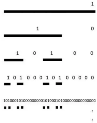
2.1. Generation of the Cantor-set by an L-system. ... 35
2.2. D0L-system for simple simulation of the development of a plant. ... 36
2.3. The first steps of the simulation of the growing of the plant. ... 36
2.4. The classes of L-languages, their hierarchy and their relation to the Chomsky-hierarchy (blue colour) in a Hasse diagram. ... 46
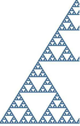
2.5. Give a D0L-system that generates the fractal shown here. ... 48
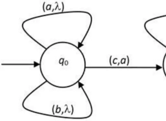
3.1. The WK-automaton accepting the language {wcw | w ∈ {a,b}*}. ... 62
3.2. The WK-automaton accepting the language {anbmcnbm | n,m > 0}. ... 63
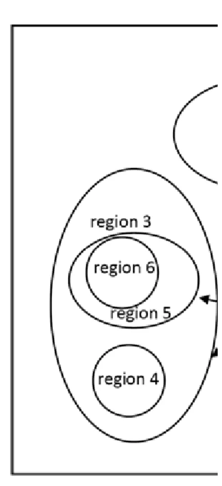
3.3. Tree structure of a membrane system. ... 71
3.4. Example for P automaton. ... 72
3.5. Von Neumann- and Moore-neighbourhood (green and blue colours, respectively), the numbers show a possible order of the neighbourhood set. ... 75
3.6. An example for the evolution of cellular automaton with Wolfram-number 160 from a given initial configuration. ... 78
3.7. Automaton with Wolfram-number 4 obtains a stable configuration. ... 78
3.8. Automaton with Wolfram-number 108 leads to configurations that are periodic (in time). ... 79
3.9. The evolution of the automaton with Wolfram-number 22 starting from a random-like configuration. 79 3.10. An example for the evolution of automaton with Wolfram-number 110. ... 79
3.11. Still lifes: stable pattern(s) in the game of life. ... 82
3.12. The pattern ''gun'' that produces ''gliders''. ... 83
3.13. A Garden of Eden. ... 85
4.1. Graph of commutation and graph of dependency. ... 88
4.2. A non-connected trace ... 89
4.3. Representation of a semi-commutation. ... 90
4.4. In the two-dimensional square grid the shortest paths form a trace, since the order of the steps is arbitrary, all words with vector (5,3) give a shortest path. ... 92
4.5. The graph of the finite automaton with translucent letters that accepts the language {w∈{a,b,c}*| |w|a = |w|b = |w|c} (the translucent letters are marked by red colour). ... 95
4.6. The graph of the automaton accepting the correct bracket-expressions (Dyck language). ... 96
5.1. Petri net with sequential run with initial marking. ... 102
5.2. A parallel run in Petri net with initial marking. ... 102
5.3. Conflict situation, modelling a non-deterministic choice. ... 103
5.4. Example for reachability graph. ... 105
5.5. A (simplified) model of bike assembly. ... 109
5.6. Modelling chemical reactions. ... 110
5.7. Various liveness properties in a place-transition net. ... 112
5.8. A place-transition Petri net with its initial marking. ... 114
5.9. Covering graph for the net given in Figure 5.8. ... 114
5.10. Eliminating chain-transition. ... 116
5.11. Eliminating chain place. ... 116
5.12. Reduction of double places. ... 117
5.13. Reduction of double transitions. ... 117
5.14. Eliminating loop place. ... 118
5.15. Eliminating loop transition. ... 118
5.16. (symmetric) confusion. ... 120
5.17. A free-choice net. ... 121
5.18. A hierarchic model having subnets for a place and a transition. ... 123
6.1. The flow chart of bubble sort. ... 134
6.2. The flow chart of parallel bubble sort; J is a set type variable. ... 134
6.3. Input actor. ... 135
6.4. Output actor. ... 135
6.5. Adder actor. ... 135
6.6. Condition generator. ... 135
6.7. Port splitter; the output token of A appears at the input ports of B and C in the same time. ... 136
6.8. Collector actor; the output token of A or B appears on the input if it becomes empty. ... 136
6.9. Gate actor; if a signal arrives from B, then A is transferred from the input port to the output port. 136 6.10. Selecting the minimum; X = min{xX1, xX2, xX3, xX4}. ... 136
6.11. The data flow graph of bubble sort. ... 136
6.12. The dependency graph of the solver of quadratic equations. ... 139
6.13. The syntactical dependency graph of the program. ... 139
6.14. Expressing deeper dependency for the same code. ... 140
A táblázatok listája
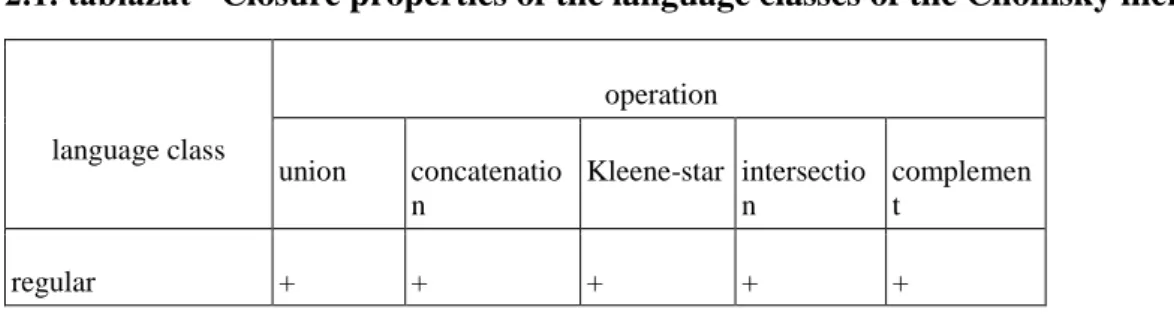
2.1. Closure properties of the language classes of the Chomsky hierarchy. ... 26
Introduction
The classical computing paradigms (Turing machine, Chomsky-type generative grammars, Markov normal algorithms, etc.) work entirely in a sequential manner as the Neumann-type computers do, too. Among the theoretical models parallel computing models have appeared in the middle of the last century, but their importance were mostly theoretical since in practice only very few special architecture machines worked in a parallel way (and their parallelism was also very limited, in some cases the sequential simulation was faster than the parallel execution of the algorithm). In the past 10-15 years, however, Moore's law about the increasing computational powers still works notwithstanding that the producing techniques are very close to their physical limits. This is done by a new way of developments. Instead of the earlier trends, increasing the speed of the CPU, the new trend uses parallel computing. Nowadays almost everywhere only parallel architectures are used and we can meet almost only them in the market. Desktop, portable, laptop, netbook computers have several processors and/or cores, they are equipped with special (parallel) GPU's; moreover smart phones and tablets also use parallel processors. We can use FPGA's, supercomputers, GRID's and cloud computing technologies.
Therefore it is necessary for a programmer, a software engineer or a electronic engineer to know the basic parallel paradigms. Besides the (traditional) Silicon-based computers, several new computing paradigms have emerged in the past decades including the quantum computing (that is based on some phenomena of quantum mechanics), the DNA computing (the theoretical models using DNA's and also the experimental computations), the membrane computing (P-systems) or the interval-valued computing paradigm. These new paradigms can be found in various (text)books (we can refer to the book Benedek Nagy: Új számítási paradigmák (Bevezetés az intervallum-értékű, a DNS-, a membrán- és a kvantumszámítógépek elméletébe); New computing paradigms (Introduction to the interval-valued, DNA, membrane and quantum computing), Typotex, 2013, in Hungarian);
in the present book we consider mostly the traditional models.
There are several ways to define and describe traditional computing methods, algorithms and their models.
Traditonal forms to give algorithms are, e.g, automata, rewriting systems (such as grammars)…
The structure of the book is as follows. In the first part we give the basic methods to analyse algorithms and basic concepts of complexity theory. Then we analyse the parallel extensions of the traditional formal grammars and automata: starting with the simplest Indian parallel grammars and D0L-systems, through on the Russen parallel grammars and the scattered context grammars to ET0L and IL systems. The cooperative distributed (CD) and parallel communicating (PC) grammar systems are also presented. Part III is about parallel automata models. We will show the 2-head finite automata (WK-automata), both the variants in which both heads go to the same direction and the variants in which the 2 heads are going to opposite direction starting from the two extreme of the input. At m-head finite automata we distinguish the one-way models, where every head can go only from the beginning of the input to its end, and the two-way variants where each head can move in both directions. We also present the simplest P-automata and give an overview on cellular automata. In part IV traces and trace languages are shown, we use them to describe parallel events. Then, in part V the Petri-nets are detailed: we start with elementary (binary) nets and continue with place-transition nets. Finally some more complex nets are recalled, shortly. Part VI is about parallel programming: we show some entirely parallel algorithms and also analyse how sequential algorithms can be changed to their parallel form. Finally, instead of a summary, the two basic forms of the parallelism are shown.
In this way the reader may see several parallel models of algorithms. However the list of them is not complete, there are some other parallel models that we cannot detail due to lack of space, some of them are the neural networks, the genetic algorithms, the networks of language processors, the automata networks, the (higher- dimensional) array grammars, etc. Some of them are closely related to the models described in this book, some of them can be found in distinct textbooks.
This book is written for advanced BSc (undergraduate) students and for MSc (graduate) students and therefore it assumes some initial knowledge. However some chapters can also be useful for PhD students to extend their knowledge. There is a wide list of literature given in the book and thus the reader has a good chance to get a deep theoretical and practical knowledge about the parallel models of the algorithms.
Parts I and VI are written by Tamás Herendi, while parts II, III, IV, V and VII are written by Benedek Nagy.
The authors are grateful to Szabolcs Iván for his help by reading and reviewing the book in details. They also thank the TÁMOP project, the Synalorg Kft and the publisher (Typotex Kiadó) their help and support.
Debrecen, 2013.
The authors
1. fejezet - Methods for analysis of algorithms
1.1. Mathematical background
1.1.1.1.1. The growth order of functions
In the following chapters, according to complexity theory considerations, we will have to express the order of growth of functions (asymptotic behavior) in a uniform way. We will use a formula to express the most important, the most steeply growing component of the function.
Let and denote the set of natural and real numbers, respectively, and let + denote the set of positive real numbers.
Definition: Let f: → + be a function.
The set O(f) = {g ⊣| ∃c > 0, N > 0, g(n) < c ⋅ f(n), ∀ n > N}
is called the class of functions which belongs to the order of growth of function f.
If g ∈ O(f), then we say that "g is a big O f" function.
Remark: In order to make the "order of growth" explicit, we may suppose that f is monotone increasing, but it is not necessary. This assumption would make a lot of observations unnecessarily complicated, thus it would become harder to understand.
Based on the definition, the most evident example is that a function bounds from above the other. However, it is not necessary. In the following we will observe through several example graphs what the growth order expresses, at least for at first sight.
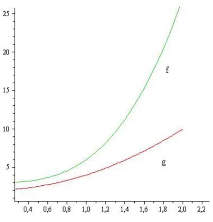
Example (the order of growth; g(n) < f(n))
Supposing that g(n) < f(n), ∀ n ∈ , the conditions of the definition are satisfied with the choice of c = 1, N = 1.
1.1. ábra - The orders of growth g(n) < f(n).
Example (the order of growth; ; g(n) < f(n), if n > N)
Supposing that g(n) < f(n), ∀ n > N, for small n's we do not care about the relation of the functions.
1.2. ábra - The orders of growth g(n) < f(n), ha n > N.
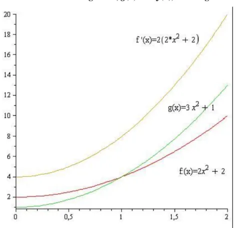
Example (the order of growth; g(n) ∈ O(f(n)) are general)
In the example g(n) > f(n), ∀ n ∈ , but if we multiply f by a constant, it is not smaller than g anywhere. g(n)
∈ O(f(n)). for the general case.
1.3. ábra - The orders of growth; g(n) ∈ O(f(n)) for the general case..
Remark: Instead of g ∈ O(f) we often use the traditional g = O(f) notation.
Properties
1. f(n) ∈ O(f(n)) (reflexivity)
2. Let f(n) ∈ O(g(n)) and g(n) ∈ O(h(n)). Thus f(n) ∈ O(h(n)) (transitivity)
Proof:
1. Let c = 2 and N = 0. Since f(n) > 0 for all n ∈ , thus f(n) < 2f(n) for all n > 0. √
2. Let c1 and N1 be such that f(n) < c1⋅ g(n), if n > N1 and let c2 and N2 be such that g(n) < c2 ⋅ h(n), if n > N2. If we set c = c1 · c2 and N = max{N1, N2}, then we get f(n) < c1 · g(n) < c1(c2 · h(n)) = c · h(n), if n > N1 and n > N2, which means n > N. √
Remark:
1. The notion of transitivity expresses our expectation that if the function f is increasing faster than g, then it is increasing faster than any function which is slower than g.
2. The order of growth is neither a symmetric nor an antisymmetric relation.
3. For the symmetry ( g ∈ O (f) ⇒ f ∈ O(g) ) the functions f = n and g = n2 and for the antisymmetry ( g ∈ O(f), f ∈ O(g) ⇒ f = g ) the functions f = n és g = 2n are counterexamples.
Further properties:
5. Let g1 ∈ O(f1) and g2 ∈ O(f2). Then g1 + g2 ∈ O(f1 + f2) . 6. Let g1 ∈ O(f1) and g2 ∈ O(f2). Then g1 ⋅ g2 ∈ O(f1 ⋅ f2) .
7. Let f be monotone increasing and f(n) > 1 ∀ n ∈ and ∈ O(f) . Then log(g) ∈ O(log(f)).
Proof:
5. Assume that c1, c2 and N1, N2 are such that
∀ n > N1 : g1(n) < c1 ⋅ f1(n) and
∀ n > N2:g2(n) < c2 ⋅ f2(n).
Let c = max{c1, c2} and N = max{N1, N2}. Then
∀ n > N: g1(n) + g2(n) < c1 ⋅ f1(n) + c2 ⋅ f2(n) < c ⋅ (f1(n) + f2(n)). √ 6. As before, assume thatc1, c2 and N1, N2 are such that
∀ n > N1 : g1(n) < c1 ⋅ f1(n) and
∀ N2 : g2(n) < c2 ⋅ f2(n).
Let c = c1 ⋅ c2 and N = max{N1, N2}. Then
∀ n > N: g1(n) ⋅ g2(n) < c1 ⋅ f1(n) ⋅ c2 ⋅ f2(n) < c ⋅ f1(n) ⋅ f2(n). √
7. Assume that c and N are such that ∀ n > N: g(n) < c ⋅ f(n). Without loss of generality we may assume that c
> 1. Since the function log(. ) is strictly monotone increasing,
∀ n > N:log(g(n)) < log(g(n) < log(c ⋅ f(n)) = log(c) + log(f(n)).
Since c, f(1) > 1, thus log(c), log(f(1)) > 0. Let
Because of the monotonity of f, we have f(1) < f(n) ∀ n > 1 and log(c) + log(f(n)) =
c’ ⋅ log(f(n))
∀ n ∈ . √ Corollary:
1. Let k1, k2 ∈ +! Then
if and only if k1 ≤ k2.
2. Let k1, k2 ∈ +! Then k1n ∈ O(k2n) if and only if k1 ≤ k2. 3. Let k∈ +! Then nk ∈ O(2n) and 2n ∉ O(nk).
4. Let k ∈ +! Then log(n) ∈ O(nk).
Proof:
The Corollaries 1, 2, 3 and 4 can be simply derived from Properties 5, 6 and 7. √
Remark:
Some particular cases of Corollary 1:
1. n ∈ O(n2) and more generally 2. nk ∈ O(nk+1) for all k > 0
To express the order of growth more precisely, we may use other definitions as well. Some of these will be given in the next few pages, together with the observation some of their basic properties.
Definition: Let f: → + be a function. The set Θ(f) = {g| ∃ c1, c2 > 0, N > 0, c1 · f(n) < g(n) < c2 · f(n) if n >
N} is called the class of functions belonging to the exact growth order of f.
Properties:
Let g, f: → + be two functions. Then
1. g ∈ Θ(f) if and only if g ∈ O(f) and f ∈ O(g) and 2. g ∈ Θ(f) if and only if f ∈ Θ(g).
Proof:
1. By the definition of the relations g ∈ O(f) and f ∈ O(g) we know that ∃ c1 > 0 és N1 > 0, such that g(n) < c1 ⋅ f(n) if n > N1 and f(n) < c2 ⋅ g(n) ifn > N2 .
Let = max{N1, N2},
and c’2 = c1.
By the inequalities above we get c1’ · f(n) < g(n) < c2’ · f(n), if n > N . √
2. By 1, g ∈ Θ(f) if and only if g ∈ O(f) and f ∈ O(g). Swapping the roles of f and g, we get f ∈ Θ(g) if and only if g ∈ O(f) and f ∈ O(g). The two equivalences imply the statement of the theorem. √
Definition: Let f: → + be a function. The set o(f) = {g| ∀ c > 0, ∃ N > 0, g(n) < c · f(n), ha n > N} is called the class of funtions having strictly smaller growth order than f.
If g ∈ o(f), we say that "g is a small o f" function.
Properties:
Let g, f: → + be two functions. Then 1. g(n) ∈ o(f(n)) if and only if
2. O(f(n)) = Θ(f(n)) ∪ o(f) and 3. Θ(f(n)) ∩ o(f(n)) = ∅.
Proof:
1. Let c > 0 and Nc > 0 be such that g(n) < c · f(n) , if n < Nc. Then
if n > Nc, thus for all small c > 0 the Nc bound can be given to satisfy
for all n > Nc. By the definition of limit this means exactly that
Conversely,
yields that ∀ c > 0 ∃ N > 0, such that
if n > N. Multiplying this by f(n) we get the statement √
2. By the definitions it is clear that o(f(n)) ⊆ O(f(n)) and Θ(f(n)) ⊆ O(f(n)).
Let (n) ∈ O(f(n))\Θ(f(n)).
Since g(n) ∈ O(f(n)), thus by definition ∃ c2 > 0 and N2 > 0 , such that g(n) < c2 < c2 · f(n) if n > N2 .
Since g(n) ∉ Θ(f(n)), by the previous inequality and the definition ∀ c1 > 0 ∃ Nc1 > 0 such that c1 · f(n) ≥ g(n) if n > Nc1, which is the statement to prove.√
3. In an indirect way, assume that Θ(f(n)) ∩ o(f(n)) ≠ ∅. Then ∃ g(n) ∈ Θ(f(n)) ∩ o(f(n)). For this g by definition ∃ c1 > 0 and N1 > 0, such that
c1 · f(n) < g(n) if n > N1 and ∀ c > 0, ∃ Nc > 0 such that g(n) < c · f(n), if n > N . Let N’ = max{N1, Nc1}.
For this N’
c1 · f(n) < g(n) and g(n) < c1 · f(n), if n > N’, which is a contradiction. √
In the follwing we need to describe the input of a problem and thus we define the following concepts:
We start by the alphabet and by the formal languages (over the alphabet).
Definition: An arbitrary nonempty, finite set of symbols is called an alphabet, and denoted by T; the elements of T are the letters (of the alphabet). The set of words obtained from the letters of the alphabet including the empty word λ is denoted by T*. L is a formal language over the alphabet T if L⊆T*. The length of a word in the form w = a1…an (where a1,…,an∈T) is the number of letters the word contains (with multiplicity), formally:
|w|=n. Further, |λ|=0.
Further we will denote the aphabet(s) by ∑, T and N in this book.
1.1.1.1.2. Complexity concepts
When we are looking for the algorithmic solution of a particular problem, in general it is not fully defined. It involves some free arguments and thus we deal with a whole class of problems instead. If, for example, the task is to add two numbers, then there are so many free parameters that we cannot find a unique solution. (For such a general task we may have for example to compute the sum or π + e.)
To make more strict observations, we have to tell more precisely what the problem is we want to solve. In the simplest way (and that could be the most common way), we represent the problems to be solved by words (sentences), thus the class of problems can be interpreted as a language containing the given sentences.
The solver algorithm during the solution may use different resources and the quantity of these resources, of course, depends on the input data. For the unique approach it is usual to distinguish one of the properties of the input - perhaps the most expressive -, the quantity or the size. If we know this information, we may define the quantity of the necessary resources as a function of it. After all, we may use further refinements and observe the need for these resources in the worst case, at average or with some other particular assumption. For more simplicity (and to make the calculation simpler), usually we do not describe the exact dependency, only the order of growth of the dependency function. (Of course the phrase "exception proves the rule" stands here as well: sometimes we can define quite exact connections.)
Definition: Resource complexity of an algorithm:
Let Σ be a finite alphabet, an algorithm and e a given resource. Assume that executes some well defined sequence of steps on an arbitrary w ∈ Σ* input that needs E(w) unit of the resource type e.
Then the complexity of the algorithm that belongs to resource e:
fe(n) = max{E(w)| w ∈ Σ*, |w| ≤ n}.
In the following we will look over the complexity concepts that belong to the most important resources. The exact definitions will be given later.
1. Time complexity
This is one - and the most important - property of the algorithms. With the help of time complexity we can express how a given implementation changes the running time with the size of the input. In general it is the number of operations we need during the execution of an algorithm.
Remark: We have to be careful with the notion of time complexity as the different definitions can give different values.
One of the most precise models for the description of algorithms is the Turing machine. The time complexity can be expressed precisely by it, but the description of the algorithms are rather complicated.
The RAM machine model is more clear and is closer to programming, but gives the opportunity to represent arbitrary big numbers in the memory cells and we can reach an arbitrary far point of the memory in the same time as the closer ones.
In practice the most common algorithm description method is the pseudo code. The problem is that in this case we consider every command having a unit cost and this can change the real value of the time complexity.
2. Space complexity
It expresses the data storage needs of the algorithm while solving the problem. We express that with a basic unit as well.
Remark: The Turing machine model gives the most exact definition in this case, too. However, the RAM machine still has the problem that in one cell we can represent an arbitrary big number. If not every memory cell contains valuable data, then the space needed could be either the number of the used cells or the maximal address of an accessed cell. (An upper bound on the space complexity of a Turing machine can be obtained from the largest address multiplied by the length of the largest number used by the corresponding RAM machine.) In other models with network features, the real space complexity can be hidden because of the communication delay.
3. Program complexity
It is noteworthy, but in the case of sequential algorithms it does not have that big importance. It expresses the size of the solving algorithm, by some elementary unit.
Remark: Contrary to these two former properties, the program complexity is independent from the size of the problem. In practice the size of program, due to physical bounds, is not independent from the input size. This is because of the finiteness of computers. If the size of the input data is exceeding the size of the memory, then the program should be extended by proper storage management modules.
We can represent the nonsequential algorithms in several models as well. In each model new complexity measurements can be defined as a consequence of parallelity. Just as before, we will give the number of necessary resources in terms of an elementary unit.
1. Total time complexity
Basically this is the time complexity of sequential algorithms, we express it with the number of all the executed operation and data movement.
2. Absolute time complexity
It gives the "time" that has passed from the beginning to the end of the execution of the algorithm, expressed by the number of commands. The operations executed simultaneously are not counted as different operations.
3. Thread time complexity
If it can be interpreted in the given algorithm model, it gives the different threads' time complexity. This is typically used in models describing systems with multiple processors.
4. Total space complexity
Similarly to the total time complexity, it is the complete data storage resource need of an algorithm.
5. Thread space complexity
It is the equivalent of thread time complexity, if independent computation threads and independent space usage can be defined.
6. Processor complexity (~number of threads)
If in the model we can define some computing unit, processor complexity expresses the quantity of it.
7. Communication complexity
If the computation described by the model can be distributed among different computing units, each of them may need the results given by the other units. The measure of this data is the communication complexity.
A property, related to the complexity concepts is the parallel efficiency of an algorithm. We can describe by the efficiency how the algorithm speeds up the computation by parallelizing.
Definition: Let be an algorithm, T(n) be the total time complexity and let t(n) be the absolute time complexity of it. The value
is the algorithm's parallel efficiency.
Between the parallel efficiency and the processor complexity the following relation holds.
Theorem: Let be an algorithm, H(n) be the parallel efficiency of the algorithm, P(n) be the processor complexity. Then (n) ≤ P(n) .
Proof: Because of the absence of the exact definitions we will only see the principle of the proof.
Let T(n) be the total time complexity and let t(n) be the absolute time complexity of the algorithm.
If the algorithm works with P(n) processor for t(n) time, the total time complexity cannot be more than P(n) · t(n).
Transforming these we get T(n) ≤ P(n) · t(n)
which was to be proved. √
Definition: Let be an algorithm, P(n) be its processor complexity and let H(n) be its parallel efficiency. The value
is the algorithm's processor efficiency.
Remark: The processor efficiency expresses how much of the operating time of the processors uses the algorithm during the operation. The value can be at most 1.
Limited complexity concepts:
As extensions of theoretical complexities, we can define practical or limited complexities. Then we keep one or more properties of the algorithm between bounds – typical example is the limitation of the number of processors or the used memory – and we investigate only on the key parameters. This is proportional to the observation of complexity of programs used in everyday life, as the implemented algorithms only work on a finite computer.
1.2. Parallel computing models
Between the different complexity concepts there is some relation. How can we express all these in a theoretic way?
The well known Space Time theorem gives the relation between space and time complexity in the case of deterministic single tape Turing machine.
Previously we set up a relation between the total time complexity, the absolute time complexity and the processor complexity of the algorithms.
In this chapter, with a special Turing machine model, we will concretize the complexity concepts defined in chapter 2 and we also define the relation between them.
The Turing machine is one of the oldest models of computing. This model can be used very efficiently during theoretical observations and for determining complexity values in case of certain sequential algorithms. What about parallel algorithms? The Turing machine model, because of its nature, is perfect for describing parallel algorithms, but from a practical point of view (programming) cannot necessarily solve the problems or analyze some particular complexity issues.
Those who have some experience in informatics, have some idea what an algorithm is. In most cases, we can decide whether the observed object is an algorithm or not. At least in "everyday life". It is almost clear that a refrigerator is not an algorithm. A lot of people associate to a computer program when it hears about algorithms
and this association is not completely irrational. However it is not obvious that a medical examination or even walking are not algorithms.
The more we want to refine the concept, the more we arrive to difficulties. Anyway, we have the following expectations of algorithms:
An algorithm has to solve a well determined problem or sort of problem.
An algorithm consists of finitely many steps, the number of these steps is finite. We would like to get a solution in a finite time.
Each step of the algorithm has to be defined exactly.
The algorithm may need some incoming data that means a special part of the problem to be solved. The amount of the data can only be finite.
The algorithm has to answer the input. The answer has to be well interpretable and finite of course.
Apparently, the more we want to define the notion of an algorithm, the more uncertainty we have to leave in it.
The most problematic part is the notion of "step". What does it mean "exactly defined"? If we give an exact definition, we restrict the possibilities.
People have tried to find an exact definition to the algorithm in the first half of the last century as well. As a result several different notions were born, such as lambda functions, recursive functions, the Markov machine and the Turing machine. As they are well defined models, we can have the impression that they are not appropriate for replacing the notion of algorithm.
One may assume that the above models are equivalent, which means that every problem that can be solved in one of the models, can be solved in the others as well.
To replace the notion of algorithm, until now, no one has found any models that are more complete then the previous ones. In this section we will pay attention to the Turing machine model as it is the clearest, easily interpretable and very expressive. However it is not very useful while modeling the recently popular computer architectures.
With Turing machines we can easily express the computability, the notion of solving the problem with an algorithm and we can determine a precise measure of the complexity of algorithms or of the description of the difficulty of each problem.
The name Turing machine is referring to the inventor of the model, A. Turing (1912-1954). The actual definition has plenty of variations with the same or similar meaning. We will use the clearest one which is one of the most expressive.
For even trying to describe the algorithm with mathematical tools, we have to restrict the repertoire of the problems to be solved. We have to exclude for example the mechanical operations done on physical objects of the possibilities. It does not mean that this kind of problems cannot be solved in an algorithmic way, it is just that instead of the physical algorithm we can only handle the mathematical model, and turn them into physical operations with the necessary interface. In practice, basically it always works like that, since we cannot observe the executed algorithms and the results of the corresponding programs themselves.
Thus we can assume that the problem, its parameters and incoming data can be described with some finite representation. Regarding this, in the following we will give the input of an algorithm (i.e. the description of the problem) as a word on a given finite alphabet and we expect the answer in the same way as well. So we can consider an algorithm as a mapping that transforms a word to another. It is clear that we can specify algorithms that do not have any reactions to certain inputs, which means that they do not specify an output (the so called partial functions). We can imagine some particular algorithms that despite the infinite number of the incoming words they can only give a finite number of possible answers. For example there is the classical accepting (recognizing) algorithm, which answers with yes or no depending on the value of the input (accepts or rejects the input).
In the following we will see that this accepting problem may seem easy, but it is not. There exist such kinds of problems that we cannot even decide whether they can be solved or not.
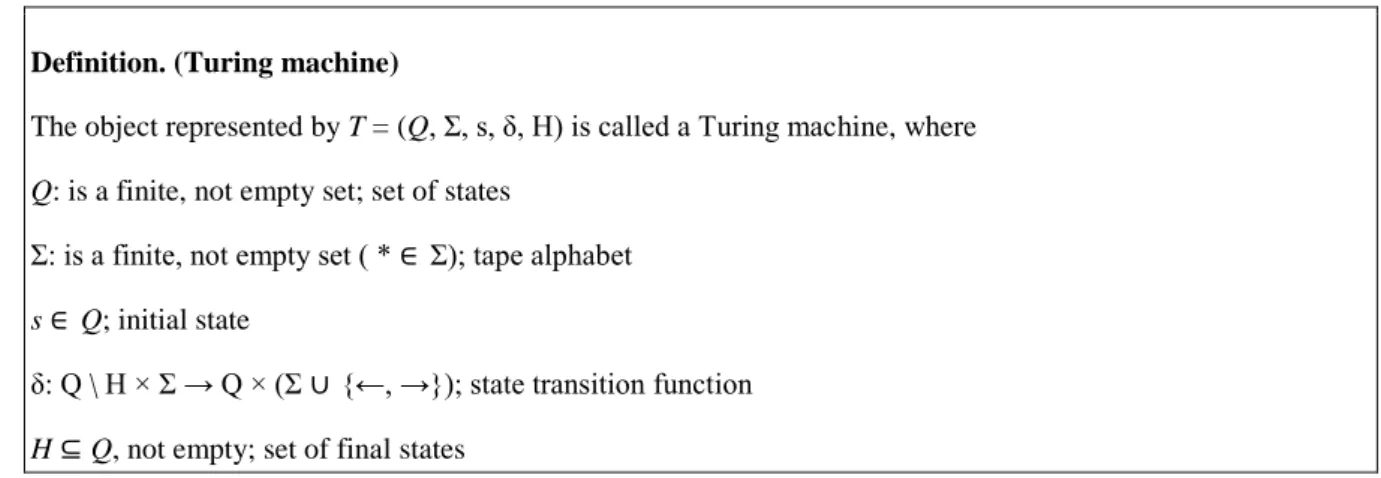
Definition. (Turing machine)
The object represented by T = (Q, Σ, s, δ, H) is called a Turing machine, where Q: is a finite, not empty set; set of states
Σ: is a finite, not empty set ( * ∈ Σ); tape alphabet s ∈ Q; initial state
δ: Q \ H × Σ → Q × (Σ ∪ {←, →}); state transition function H ⊆ Q, not empty; set of final states
This formal definition above has to be completed with the corresponding interpretation. The following
"physical" model will be in our minds:
In the imaginary model the Turing machine has 3 main components:
1. State register: It consists of one element of Q, we can determine the behavior of the Turing machine with it.
The stored value is one of the arguments of the state transition function.
2. Tape: It is infinite in both directions (in certain interpretations it can be expanded infinitely), it is a sequence of discrete cells (storing elements of the tape alphabet) of the same size. Each cell contains an element of the alphabet Σ. It does not influence the interpretation of the Turing machine that consider the tape infinite in one or both directions (or infinitely expandable) as in all cases we assume that on the tape we only store a single word of finite length. On the rest of the tape the cells contain the dummy symbol: ∗ . (In certain interpretations this ∗ symbol is the letter denoting the empty word.)
3. Read write head: It sets up the relation between the tape and the status register. On the tape it always points to a particular cell. The Turing machine can read this cell and write in it. During the operation the read write head can move on the tape.
1.4. ábra - Turing machine.
The operation of the Turing machine: The Turing machine, during its operation, executes discrete steps. Let's assume that it implements every step in a unit time (and at the same time).
a.) At the start, the status register contains the initial state s, while on the tape the input word w can be found.
The read write head points to the cell preceding the first letter.
b.) During a step, it reads the sign under the R/W head, with the transition function δ and the read sign it defines the new state and the new sign to be written on the tape or movement value of the R/W head. (Or it writes on the tape or it moves its head.) It writes the new internal state in the status register, the tape sign in the cell of the tape which is under the R/W head. Then it owes the R/W head to the next cell.
c.) If the content of the status register is a final state, then it stops and the output is the word written on the tape.
(There is a definition of the Turing machine which says it stops as well when the transition function is not defined on the given state and read letter, but this case can be eliminated easily, if we assume that the value of state transition function is a final state every time we do not tell it exactly.)
According to the interpretation kept in mind we need an "operation" that is exact and mathematically well determined. The following definitions will describe it.
Definition:
Let T = (Q, Σ, s, δ, H) be a Turing machine. Any element K ∈ Q × ((Σ* × Σ × Σ*)\( Σ + × {∗} × Σ+)) is a configuration of T .
According to the definition a configuration is a quadruple: K = (q, w1, a, w2), whereq is a state, w1is the space on the tape before the R/W head, a is the letter under the R/W head and w2 is the space on the tape after the R/W head. Although, by the definition of transition function it would be possible, but since we have excluded the elements of Q × Σ+ × {∗} × Σ+, thus the configurations with empty cells under the R/W head are not valid if both before and after nonempty cells can be found.
Remark: If it does not cause any problem in the interpretation, for more simplicity in the configuration we won't tell the exact place of the R/W head. Then its notation will be the following:
K = (q, w) ∈ Q × Σ*,
where q is the state of the Turing machine and w is the content of the tape.
Definition: Let T = (Q, Σ, s, δ, H) be a Turing machine and K = (q, ,w1, a, w2) be a configuration of T.
We say that T goes in one step (or directly) from K to configuration K’ (with signs K ⊢K’), if K’ = (q’, w1’, a’, w2’) and exactly one of the following is true:
1) w1’ = w1
w’2 = w2
δ(q, a) = (q’, a’), where a, a’ ∈ Σ, q Σ Q\H and q’ Σ Q.
(overwrite mode) 2) w1’ = w1 · a w2 = a’ · w2’
δ(q, a) = (q’, →), where a ∈ Σ, q Σ Q\H and q’ ∈ Q.
( right shift mode )
3) w1= w1’ · a’
w2’ = a · w2
δ(q, a) = (q’, ←), where a ∈ Σ, q ∈ Q\H and q’ ∈ Q.
( left shift mode )
Definition: Let T = (Q, Σ, s, δ, H) be a Turing machine and C = K0, K1, …, Kn, …, be a sequence of configurations of T.
We say that C is a computation of the Turing machine T on the input word w, if 1. K0 = (s, λ, a, w’), where w = aw’;
2. Ki ⊢ Ki+1 , if there exists a configuration that can be reached from Ki directly (and because of uniqueness, it is Ki+1);
3. Ki = Ki+1, if there is no configuration that could be reached directly from Ki .
If h ∈ H for some Kn = (h, w1, a, w2), then we say that the computation is finite, T stops in the final state h. Then we call the word w’ = w1 · a · w2 the output of T. Notation: w’ = T(w).
If in case of a w ∈ Σ* the Turing machine T has an infinite computation, then we do not interpret any outputs.
Notation: (w) = ∅. (Must not confuse with the output (w) = λ .)
Definition (Recursive function):
We call the function f: Σ* → Σ* recursive, if ∃ T Turing machine such that ∀ w ∈ Σ* f(w) = T(w).
Definition: The object represented by the quintuple T = (Q,, Σ, s, ∆, H) is called a Super Turing machine, if Q: finite, nonempty set; (set of states)
Σ finite, nonempty set, ∗ ∈ Σ; (tape alphabet) s ∈ Q; (initial state )
∆: Q\H × Σ* → Q × (Σ ∪ {←, →})*; (transition function) recursive, i.e. is computable by a simple Turing machine H ⊆ Q, nonempty set; (set of final states)
The Super Turing machine has an infinite number of tapes and among these, there are a finite number of tapes containing data, moreover each such tape contains a finite amount of data only. All of them has their own a R/W head which move independently from each other.
1.5. ábra - Super Turing machine
We define the notion of configuration and computation analogously to the case of Turing machines.
Definition: Let T = (Q, Σ, s, ∆, H) be a Super Turing machine. K is a configuration of T such that K = Q ×((Σ* × Σ × Σ*) \ (Σ+ × {∗} × Σ+))*.
Remark: If it does not cause any interpretation problems, for more simplicity in the configuration we don't mark the exact place of the R/W head. In this case the notation will be the following:
K = (q, w1, …, wk) ∈ Q × (Σ*)*, where 1 ≤ k. Here q is the state of the Turing machine and w1, …, wk are the contents of the first k tapes.
Definition: Let T = (Q, Σ, s, ∆, H) be a Super Turing machine and K = (q, (w1,1, a1, w2,1), …, (w1,k, ak, w1,k)) be a configuration of T. (Only the first kk tapes contain any information.)
We say that T goes in one step (or directly) from K to K’ (notation K ⊢ K’), if K’ = (q’, (w’1,1, a’1, w’2,1), …, (w’1,l, a’l, w’2,1)) ,
q ∈ Q\H and q’ ∈ Q, A = a1 … ak,
∆(q, A) = (q’, B) , where B = b1 … bl and
exactly one of the following is true, for all∀ 1 ≤ i ≤ max {k, l}:
1) w’1,i = w1,i
w2,i = w2,i
bi = a’i.
2) w’1,i = w1,i · ai
w2,i = a’i · w2,i
bi = →
3) w1,i = w’1,i · a’i
w’2,i = ai · w2,i
bi = ←.
Definition: Let T = (q, Σ, s, ∆, H) be a Super Turing machine and
C = K0, K1, …, Kn, … be a sequence of configurations of T.
We say that C is a computation of the Super Turing machine T on the input word w, if 1. K0 = (s, λ, a, w’), where w = aw’ (in case w = λ we have a = ∗ and w’ = λ);
2. Ki ⊢ Ki+1, if there exists a configuration directly reachable from Ki (and because of uniqueness Ki+1);
3. Ki = Ki+1, if there is no configuration directly reachable from Ki .
If Kn = (h, w1, w2, …, wk) with h ∈ H, then we say that the computation is finite and T stops in the final state h . By default, w1 is the output of T. Notation: w1 = T(w). In other cases, the content of the output tape(s) is the result of the computation.
If the Super Turing machine T has an infinite computation on w ∈ Σ*, we do not interpret the output. Notation:
T(w) = ∅. (Must not be confused with the output T(w) = λ .)
Example (positioning) T = (Q, Σ, s, ∆, H) Q = {s, h}
Σ = {0,1, ∗} H = {h}
In case of = a1 … ak : ∆(s, A) = (s, B),
where B = b1 … bk and bi =∗, if ai = ∗, and bi = ⇒ , if ai ≠∗.
∆(s, A) = (h, A) , if A = λ, namely on each tapes there is only∗ under the R/W head;
The Turing machine in the above example does only one thing: on each tape it goes to the first empty cell following a nonempty word.
Example (selection of the greatest element) T = (Q, Σ, s, ∆, H)
Q = {s, a, h}
Σ = {0, 1, x0, x1, x∗, x∗} H = {h}
Input: w1, …, wk ∈ {0, 1}*. State transition function:
In case of A = a1 … ak ∆(s, A) = (a, Ax).
∆(a, Ax) = (h, A), ha A = λ , e.g. on all the tapes there is ∗ under the R/W head;
∆(a, Ax) = (b, Bx), where ahol B = b1 … bk and bi =∗, if ai =∗, and bi = ⇒ , if ai ≠ ∗..
∆(b, Ax) = (b, B ⇒) , where B = b1 …bk és bi = xai. (The R/W head moves only on the last used tape.)
∆(b, A) = (a, Bx) , where B = b1 … bk és bi = ci , if ai = xci.
The Super Turing machine in the example writes on the first unused tape as many x signs as the lenght of the input word.
Definition: Let T be an arbitrary (Super or simple) Turing machine, k ≥ 1 and w = (w1, …, wk), where w1, …, wk
∈ Σ*.
The length of the computation of T on input w is the least n, for which the computation on the input word w, the state belonging to Kn is the final state (if it exists).
If the computation is not finite, its length is infinite.
Notation: τT(w) = n, and τT(w) = ∞ respectively.
Remark: We represent the length of the input word w = (w1, … wk) with the function l(w). Its value is l(w) = l(w1) + … + l(wk).
Definition: Let T be a (Super or simple) Turing machine.
The time complexity of T is the following function:
tT(n) = max{τT(w)|w = (w1, …, wk), where w1, …, wk ∈ Σ* and l(w) ≤ n.
Definition: Let T be an arbitrary (Super or simple) Turing machine, k ≥ 1 and = (w1, …, wk) , where w1, …, wk
∈ Σ*.
Also let K0, K1, …, Kn be the computation of T on input w. (i.e. K0 = (s, w). ) The space used by the Turing machine T on input w
σT(w) = max{|wi| Ki = (qi,wi), i = 0, …, n} . If the computation of T on input w is infinite, then σT(w) = limn→∞ max{|wi| |Ki = (qi, wi), i = 0, …, n} .
Remark: Even if the computation of a Turing machine is not finite, the space demand can be. This is typically an infinite loop.
Definition: Let T be a (Super or simple) Turing machine.
The space complexity of T is the following function:
sT(n) = max{σT(w)| w = (w1, …, wk), where w1, …, wk ∈ Σ* and (w) ≤ n}.
Definition: Let T be an arbitrary (Super or simple) Turing machine, k ≥ 1 and w = (w1, …, wk), where w1, …, wk
∈ Σ*.
Also let K0, K1, …, Kn be the computation of T on input w. (i.e. K0 = (s, w).) The processor demand of Turing machine T on input w is
If the computation of T on input w is infinite, then
Definition: Let T be a (Super or simple) Turing machine.
The processor complexity of T is the following function:
pT(n) = max{πT(w)| w = (w1, …, wk)}, where w1, …, wk ∈ Σ* and (w) ≤ n} .
Definition: Let T be a Super Turing machine and K = (q,w) be a configuration of T, where w = (w1, …, wk), k ≥ 1 and w1, …, wk ∈ Σ*.
Furthermore, let A = (a1, …, ak) be the word formed by the currently scanned symbols by the R/W heads in K and 1 ≤ i, j ≤ k.
We say that the data flows from tape j to the direction of tape i if ∃ A’ = (a’1, …, a’k), with aj ≠ a’j and al = a’l
∀ l ∈ {1, …, k} \ {j} and if B = ∆(q, A) and B’ = ∆(q, A’), then bi ≠ b’i. Accordinglyζj,i(K) = 0, if there is no data stream and ζj,i(K) = 1, if there is.
The amount of the streamed data belonging to the configuration:
According to the definition there is data stream from tape j to the direction of tape i, if we can change the letter under the R/W head on tape j such that during the configuration transition belonging to this letter the content of tape i will not be the same as in the original case.
Definition: Let T be a Super Turing machine, k ≥ 1 and w = (w1, …, wk) where w1, …, wk ∈ Σ*. Also let K0, K1, …, Kn be the computation of T on input w. (Namely K0 = (s, w). )
The communicational demand of Turing machine T on input w is ζT(w) = ∑i=0…n ζ(Ki).
The communicational bandwidth demand of Turing machine T on input w is ζT(w) = max{ζ(Ki)|Ki, i = 0, …, n}.
Definition: Let T be a Super Turing machine.
The communicational complexity of T is the following function:
zT(n) = max{ζT(w) | w = (w1, …, wk), where w1, …, wk ∈ Σ* and (w) ≤ n} . The absolute bandwidth demand of T is the following function:
dT(n) = max{ηT(w) | w = (w1, …, wk), where w1, …, wk ∈ Σ* and l(w) ≤ n}
The above definitions of the time, space and processor complexity are the clarifications of the notions of chapter Complexity concepts, in the Turing machine model.
Those notions' equivalents for the Super Turing machine:
General - Super Turing machine
Absolute time complexity ↔ Time complexity Total space complexity ↔ Space complexity Processor complexity ↔ Processor complexity
Communicational complexity ↔ Communicational complexity
Thread time complexity
The time complexity belonging to tape (thread) i can be spawned from the number of steps between the first and last significant operations, just like the general time complexity. Significant operation is the rewrite of a sign on the tape and moving the R/W head.
Total time complexity
The sum of the time complexities of threads.
Thread space complexity
The space complexity observed tapewise.
The restrictions referring to the transition function of the Super Turing machine give the different computing models and architectures.
It is clear that with the Super Turing machine model the Turing machines with one or more tapes can easily be modeled.
1.2.1.2.1. Simulation
Definition: Let 1 and 2 be algorithms possibly in different models.
We say that 1 simulates 2 if for every possible input w of 2, 1(w) = 2(w), which means that it gives the same output (and it does not give an answer, if 2 does not give it).
Let M1 and M2 be two models of computation. We say that M1 is at least as powerful as M2 if for all 2 ∈ M2
exists 1 ∈ M1 such that 1 simulates 2.
The Super Turing machine can be considered as a quite general model. With the restrictions put on the state transition function it can simulate the other models.
Examples (for each restriction)
1. If we reduce the domain of ∆ from Q\H × Σ* to Q\H × Σkwe will get to the Turing – machine with the k tape.
In this case it is not necessary to reduce the range as well, since we can simply not use the data written on other tapes.
(Mathematically it can be defined by a projection.)
2. If ∆ can be written as δ∞ where δ: Q\H × Σk → Q × (Σ ∪ {← →})k. Here, basically, the Super Turing machine can be interpreted as the vector of Turing machines with k tapes with the same behavior. In this case we store the state that is necessary for the component Turing machines on one of the tapes.
The different use of the mutual space can be modeled as well.
3. If we define the transition function such that the data to the tape i + 1 flows only from the tape i and the sign that was there before does not influence the symbol written on the tape i + 1, then the tape i + 1 can be considered as an external storage of the tape i.
4. Furthermore, if we assume the Super Turing machine in point 3 such that the data flows from the direction of the tape i + 1 to the i + 2 (but the value of the tape i + 2 depends only on i + 1, then we can model such an operation as the tape i + 1 is a buffer storage between the tapes i and i + 2 .
5. Similarly to the previous ones the concurrent use of memory can be modeled as well. With a well defined transition function, to the direction of the tape i + 1 both from the ith and the i + 2nd tape there can be a data stream. In this case the tape i + 1 is a shared memory of tapes i and i + 2.
Dropping the finiteness condition of the state space would cause the problem that a new model of algorithms would be born and with that we could solve more problems, even the ones that cannot be solved with traditional algorithms. It is because then the transition function cannot be computed by a Turing machine anymore and this way a non-computable transition function can be given.
(Example of the implementation of a nonrecursive function in case of infinite state space:
f(n) = to the longest sequence of 1 as an answer that can be given on an empty input by a Turing machine of state n.)
It is important to see that with the use of the Super Turing machine the set of solvable problems is not expanding, only the time complexity of the solution can be reduced.
Theorem: For each Super Turing machine T there exists a simple Turing machine T’ which simulates the first one.
Proof:
The proof is a constructive one, but here we only give the sketch of it.
First we have to define a simulating Turing machine, and then verify that it really solves the problem.
Let T’ be the simulating Turing machine.
We will use the first tape of T’ to store the necessary information for the proper operation. More precisely, T’
uses tape 1 to execute the operations required by the simulation of the transition function.
On the second tape there will be the inputs, then at an internal step of the computation the auxialary results will get back here.
The structure of the tapes of T’ and the operation can be described as follows:
The structure of the content of tape 2 is the following:
If the actual configuration of the simulated T is K = (q, w1,1, a1, w1,2, …, wk,1, ak, wk,2),
then on the tape the word
#w1,1 & a1 & w1,2 # … # wk,1 & ak & wk,2# can be found.
The set of states of T’ is Q’ = Q × Q1, where Q is the set of states of T and Q1 can be used to describe the simulating steps.
T’ is iterating the following sequence of steps:
1. Reads the whole 2nd tape and copies the content of the tape between the symbols & … & to the first tape; we assign an appropriate subset of Q1 to these steps.
2. After finishing the copy operation, it moves the head to the beginning of the 1st tape and switches to executive state; we assign now another appropriate subset of Q1 to these steps.
3. In the executive state it behaves like Turing machine according to ∆(q, … ). Here, obviously, another subset of Q1 is necessary.
4. After the implementation of the change of sate, it changes the content of the 2nd tape, corresponding to the result. If it finds a letter to be written, it will write it, if it finds a character that means head movement, then it will move the corresponding & symbol.
5. If the new state q’ is a final state, the simulation stops, otherwise it starts over again with the first point.
The execution of the 4th point is a little bit more complicated, since writing after the last character of the tape or erasing the last character requires an appropriate shift of the successive words.
The second part of the proof is to verify that T’ actually simulates T.
It can be done with the usual simulation proving method:
We have to prove that the computation K0, K1, … of T can be injectively embedded to the computation K’0, K’1,
… of $T'$.
Formally: ∃ i0 < i1 < i2 < …, , such that Kj and are corresponding uniquely to each other. This sequence of indices may be for example the indices of configurations at the start of the first sequence in the simulation of each step.
Essentially, this proves the theorem. √
We have to require the Super Turing machine's state transition function to be recursive, otherwise we would get a model that is too general, which would not fit to the notion of the algorithm. If the transition function is arbitrary, then it can be used for solving any problem. Even those that are not thought to be solvable in any manner.
Refining the definition, we may demand Δ to be implemented with a limited number of states on a single tape Turing machine. This does not affect the set of problems that can be solved by the Super Turing machine, but the different complexity theoretic observations will reflect more the real complexity of the problem. Otherwise, there can be a solution that gives answer to each input in 1 step.
State transition function bounded by 1 state:
Substantially, on every tape, only the content of the tape determines the behavior. It can be considered as a vector of Turing machines that are not fully independent and are operating simultaneously. Between the tapes there is no direct data stream.
State transition function bounded by 2 states:
Between the tapes there is a minimal data stream (a maximum of 1 bit). The tapes can be considered as they are locally the same.