O R I G I N A L S T U D Y
Analysis of local covariance functions applied to GOCE satellite gravity gradiometry data
Branislav Ha´bel1 •Juraj Jana´k1
Received: 20 February 2017 / Accepted: 12 October 2017 / Published online: 31 October 2017 ÓAkade´miai Kiado´ 2017
Abstract GOCE Level 2 products of corrected gravity gradients in Local North-Oriented Frame were used in this study. We analyzed four accurately measured elements of the gravity tensor, which were transformed to disturbing gravitational gradients. The investi- gation was carried out in the restricted region of dimension 20°920°covering the south part of Europe. We applied several types of analytical covariance functions in a local approximation, which have the best fit to the empirical covariances calculated from the disturbing gravitational gradients in particular sub-regions. At first, we have investigated four different types of the 1-dimensional covariance function. Obtained results show that the Gaussian covariance function approximates the empirical covariances the best from tested functions. Moreover, a time stability of calculated parameters of the covariance functions was studied by assuming GOCE data from different time periods. In the second experiment, we have compared two types of the 2-dimensional covariance function, which also enables a spatial stochastic modeling. The second study revealed that the least-squares collocation using the 2-dimensional local covariance function can produce the local grid of GOCE disturbing gravitational gradients directly from GOCE Level 2 products right below GOCE orbit, which in general fits well with the recent Earth’s global gravity field models and might have some advantages. Such local grids can be useful for specific tasks, e.g.
mutual comparing of GOCE data collected during particular time periods.
Keywords Gravity fieldLocal covariance functionGOCELeast-squares collocation
& Branislav Ha´bel
branislav.habel@stuba.sk Juraj Jana´k
juraj.janak@stuba.sk
1 Department of Theoretical Geodesy, Faculty of Civil Engineering, Slovak University of https://doi.org/10.1007/s40328-017-0208-6
1 Introduction
The quantities of the Earth’s gravity field are specified by the spatial correlation, which is widely used in applications of physical geodesy and geophysics. In general, a correlation indicates some form of similarity relation between two observables with tendency to have about same size and sign. If we consider the correlation as a function of position or time, we obtain a covariance function, which provides the basis for stochastic methods of regional and global gravity field modelling (Heiskanen and Moritz1967). The most used least-squares prediction method in physical geodesy is called least-squares collocation, where the covariance function is a crucial ingredient. It offers a powerful tool for gravity field prediction, filtering, and parameter estimation (Tscherning2010) and is also able to combine different kinds of terrestrial and satellite data. Produced local (regional) and global grids may be then used for other research, e.g. estimation of spherical harmonic coefficients derived by numerical integration.
The covariance functions can take a local and a global form (Moritz 1980). For the global covariance function, the data have to be distributed over the whole Earth to describe the stochastic properties of observables throughout the whole spectral range. Evaluation of the global covariance function requires more computational effort and large sets of data.
Various authors have been dealing with the construction and application of global covariance function, e.g. Tscherning (1976), Rapp (1978), Pail et al. (2011) and Gatti et al.
(2013). For some purposes, the local covariance function is more suitable rather than the global one. We are restricted only over a limited area instead of over the whole Earth. This approach has several advantages like handling with reduced amount of interpreted data, simpler practical determination and ensuring less computational effort. It allows carrying out more detailed studies, e.g. the interpolation problem and filtering. Local grids produced by suggested method may be more flexible than several existing global grids, e.g. Bouman et al. (2016), in terms of time span of used data or altitude. However, a true shape of the covariance function is rarely known and it depends on the region of calculation. Therefore, it must be derived directly from measured data (Jekeli 2010). The local grid is also characterized by the limited spectral resolution than the global one.
The aim of our contribution is to investigate the statistical behaviour of particular components of the disturbing gravitational tensor derived from GOCE (Gravity field and steady-state Ocean Circulation Explorer) on-orbit data. It was the first satellite gravity gradiometry (SGG) mission in the history, which was developed and led by the European Space Agency (ESA). GOCE satellite was launched on 17 March 2009 from the Plesetsk Cosmodrome in Russia. The mission finished after 4 years and 8 months on 11 November 2013, when a design life of the satellite was exceeded of about 20 months. A primary objective of GOCE was to improve a global model of the Earth’s gravity field and a geoid, both in spatial detail and accuracy, especially over the ocean (ESA 1999). Nowadays, GOCE still brings a number of applications in oceanography, geodesy, solid earth physics and many other disciplines. An extended life time and an extremely low orbit of the satellite resulted in very interesting and unique data. The spacecraft was equipped by the electrostatic gravity gradiometer with a set of three pairs of orthogonally mounted 3-axis accelerometers. It allowed to measure gravity gradients in all directions. However, only four components (VXX, VYY,VZZ, andVXZ) of the tensor were measured with ultra-high precision due to the arrangement of accelerometers. A position of the satellite was con- trolled using the on-board Global Positioning System receiver by the Satellite-to-Satellite Tracking principle. The orientation of the satellite with regard to inertial reference frame was monitored by the star-trackers. Three levels of data products are available. Level 0
includes raw data gathered by GOCE satellite. Level 1b products consist of calibrated gravity gradients measured in the gradiometer reference frame including the orbit data.
These were further processed by the European GOCE Gravity Consortium (E-GGC) to Level 2 products of corrected gravity gradients in different reference frames. More details about GOCE mission and provided products can be found in Gruber et al. (2010).
In this study, we have focused only on local covariance functions in the planar approximation. By the term ‘covariance model’ we will understand the analytical covariance function together with a small numbers of corresponding parameters. We will test different types of planar covariance models used in physical geodesy and examine both the spatial and the time dependencies of their essential parameters. Proving the usefulness of the local covariance function, we will apply the least-squares collocation method for the interpolation of the largest component of disturbing gravitational tensor to a regular grid and compare it with the recent Earth’s global gravity field models: TIM R5 (Brockmann et al.2014), EIGEN-6C4 (Fo¨rste et al.2014), and EGM2008 (Pavlis et al.2012).
2 Local covariance functions
We have restricted our study to local covariance functions described in Moritz (1980), which are well-known in physical geodesy. Let us suppose, for simplicity, that GOCE satellite is moving in the circular orbit above the reference sphereR, which lies on the spherical surface with the radiusR1(see Fig.1). Then, a local structure of the covariance function assumes a planar approximation, where the spherical surface is replaced by its tangent plane around the position of the satelliteP. If there are all positions of measured data points situated on the tangent plane, we can estimate the 1-dimensional covariance model. In this case, a stochastic dependence in the vertical direction, if exists, is neglected.
Such homogenous and isotropic covariance function depends only on planar distancesq between data points that are calculated from the spherical distances w using a simple formula:
q¼R1tanwR1w: ð1Þ
Behavior of the local covariance function can be characterized by three essential parameters (C0, n,v). A variance C0 corresponds to the covariance for the zero planar distanceq. A correlation lengthnrepresents the planar distanceq corresponding to one half of the varianceC0. The last dimensionless parametervis related to the curvature of the
Fig. 1 Planar approximation of the spherical surface with the radiusR1
covariance function at the distanceq¼0 (Moritz 1980). We have tested four different types of the 1-dimensional positive definite functions shown in Table1.
According to Moritz (1980), some 1-dimensional covariance functions can be extended to outer space by simple modification, where the altitude of data points is z[0. Such modeling is able to express the stochastic dependence in both the horizontal and the vertical direction between data points P(z) and Qðz0Þ located above the approximation plane. Altitudez of particular point can be calculated as a difference between its radial distance r and the radius of approximation sphere R1. Two types of the 2-dimensional covariance function labeled as CF5 and CF6 are listed in Table2. ConstantsA,B,bandm mentioned in Tables1and2represent additional parameters, which enable to derive the essential parametersnandv.
The essential parameters of covariance functions are either applied as theoretical values or derived from the given data. The second approach is more frequent and requires a construction of the empirical covariance function (ECF) as the first. ECF is a point-wise function and its shape primarily depends on the input data, but also on the chosen number of bins dividing data into a set of equally sized intervals. In 1-dimensional case and irregularly spaced data, the empirical covariances can be computed as:
covqaqi;j\qb
¼1 n
Xn
k¼1
ðlilÞðljlÞ
k; ð2Þ
whereliandljare measurements (e.g. gravity gradients), which correspond to the planar distancesqi;jbetween pointsi,jand satisfy conditionsqi;j2hqa;qbÞ, whereqaandqbare the limits of the particular bin. The number of all pairskof points in data set satisfying that condition is denoted as n. Taken into account stationarity of the covariance function, measured quantities are centered, i.e. reduced by the mean valuel. This process of cen- tration can be supplemented by a subtraction of normal gravity field in the sense of physical geodesy. Number of calculated empirical covariances, which corresponds to the number of bins, usually exceeds the number of unknown parameters of their analytical expression and allows applying the least-squares approach. In 2-dimensional case, the empirical covariance also depends on the sum of altitudeszþz0:
covqaqi;j\qb;ðzþz0Þa ðzþz0Þi;j\ðzþz0Þb
¼1 n
Xn
k¼1
lil ð Þljl
k; ð3Þ where the measurements li and lj also satisfy the second condition ðzþz0Þi;j2
ðzþz0Þa;ðzþz0Þb
with the limitsðzþz0Þaandðzþz0Þbof particular bin.
Table 1 The 1-dimensional local covariance functions (Moritz1980)
Covariance function Expression length Correlation Curvature parameter CF1: Gaussian covðqÞ ¼C0expðA2q2Þ n¼1A ffiffiffiffiffiffiffi
pln 2
2 ln 2 CF2: withm¼2 (Hirvonen’s) covðqÞ ¼ð1þBC20q2Þ2 n¼ ffiffiffiffiffiffiffiffiffiffi
21=21 p
B 4ð21=21Þ
CF3: withm¼1=2 covðqÞ ¼ C0
ð1þB2q2Þ1=2 n¼ ffiffi
3 p
B 3
CF4: withm¼3=2 covðqÞ ¼ C0
ð1þB2q2Þ3=2 n¼ ffiffiffiffiffiffiffiffiffiffi
22=31 p
B 3ð22=31Þ
3 Data preparation
As mentioned above, we have analyzed the corrected gravity gradients of GOCE Level 2 products (EGG_TRF_2) available via ESA GOCE Virtual Archive website (http://eo- virtual-archive1.esa.int/Index.html). Calibrated gradients in these products are given in Local-North Oriented Frame (LNOF). Geocentric position of the GOCE center of mass is defined by its spherical latitude /, longitude k and a radial distance r for a particular observation epoch. This enables to calculate the spherical distanceswbetween the pairs of data points and the altitudes above the approximation plane eventually. For more infor- mation about the EGG_TRF_2 products and the definition of LNOF system, see Gruber et al. (2010).
Our experiment has focused on four accurately measured components of the gravity tensor (VXX, VYY, VZZ, and VXZ). All gradients flagged as outliers were excluded from further analysis. A region of interest (2020) covers the south part of Europe and is restricted to /2h30N;50Ni, and k2h10E;30Ei. To study the behavior of local covariance functions in different areas, we have divided this region into four sub-regions of 1010 labeled as R1, R2, R3 and R4 (see Fig.2). Measured quantities should be corrected for a systematic part of gravity field before evaluation of empirical covariances.
Therefore, the gravity gradients were transformed to disturbing gravitational gradientsTXX, TYY,TZZ, andTXZ. These are obtained from the observed gravity tensor by subtraction of corresponding elements of normal gravity tensor by ‘Normal tensor’ software (Sˇprla´k 2012) using GRS-80 reference ellipsoid. Calculated gradients in the test region are depicted in Fig.2. Measurements from 19 January 2011 to 31 May 2011 were used for the visualization. Adjacent sub-regions are characterized by a different pattern of disturbing gravitational gradients. The amplitudes vary from -1.5 E to 1.0 E (E=Eo¨tvo¨s, 1 E = 109s2) and are the largest forTZZ component.
4 Experiment with the 1-dimensional local covariance functions
The first experiment investigates performance of the 1-dimensional covariance functions CF1, CF2, CF3 and CF4 presented in Table1. Let us assume a simplified situation, where GOCE satellite is moving on the spherical surface above the Earth. We consider that the radius of such sphere is equal to R1¼6628 km, what corresponds to the mean radial distance of the satellite in the region of interest. Then, all data points should have zero altitudes (z¼0) above the tangent plane, which locally approximates the sphere.
For all sub-regions and four components of the disturbing gravitational tensor the empirical covariances were evaluated according to Eq. (2). The planar distancesqwere divided into 25 equally spaced bins in the range from 0 to 1000 km. We have considered
Table 2 The 2-dimensional local covariance functions (Moritz1980)
Covariance function Expression length Correlation Curvature parameter CF5: withm¼1=2 covðP;QÞ ¼ C0b
ðq2þðzþz0þbÞ2Þ1=2 n¼b ffiffiffi p3
3 CF6: withm¼3=2 covðP;QÞ ¼ C0b2ðzþz0þbÞ
ðq2þðzþz0þbÞ2Þ3=2 n¼b ffiffiffiffiffiffiffiffiffiffiffiffiffiffiffiffi 22=31
p 3ð22=31Þ
measurements from 19 January 2011 to 28 February 2011. ECF of TZZ component is depicted in Fig.3. Only positive empirical covariances are displayed as the local covari- ance model is expressed by the positive definite function according to covariance function theory (Moritz1980). In addition, we should not overstep the correlation length within the interpolation procedure, where all empirical covariances get positive values.
Variances and correlation lengths for the 1-dimensional models from Table1 were estimated using the least-squares approach. In order to asses how well the estimated model approximates the empirical covariances, the coefficient of determinationRsqis calculated as (Rousseeuw and Leroy1987):
Rsq¼1 PN
i¼1ðyiy^iÞ2 PN
i¼1ðyiyÞ2; ð4Þ
where the valueyirepresents positive empirical covariance,y^iis its least-squares estimate, andyis the mean value ofy. Derived analytical covariance models forTZZcomponent are also shown in Fig.3. The best estimates are highlighted in bold. It is clearly visible that Gaussian covariance model CF1 has the best performance in all sub-regions. However,
Fig. 2 The region of interest divided into four sub-regions and scatter plot of analyzed components of the disturbing gravitational tensor along the GOCE orbit
differences between the particular models are almost negligible up to the correlation length, except for CF3 model. For completeness, mean essential parameters from four estimated models were calculated. Results involving all analyzed components of the dis- turbing gravitational tensor are summarized in Table3. It is not surprising that the esti- mates differ from one region to another, mainly for the mean variance C0. The highest values are typical for the sub-region R2 due to the most distinctive variation of disturbing
Fig. 3 The empirical covariance function of TZZ component calculated in four sub-regions and approximated by analytical covariance models CF1, CF2, CF3 and CF4 with the corresponding coefficient of determinationRsq(in brackets)
Table 3 Mean variances, corre- lation lengths and coefficients of determination calculated from the estimated covariance models CF1, CF2, CF3 and CF4 (the 1-dimensional case)
Sub-reg. Param. TXX TYY TZZ TXZ
R1 C0(E2) 0.016 0.027 0.059 0.026
n(km) 204.4 186.4 205.8 229.5
Rsq (%) 95.9 95.5 94.2 96.4 C0(E2) 0.235 0.053 0.412 0.284
R2 n(km) 215.7 186.8 213.9 222.0
Rsq (%) 92.6 93.5 92.7 91.5 C0(E2) 0.012 0.008 0.024 0.021
R3 n(km) 145.9 128.4 137.8 138.1
Rsq (%) 93.3 96.2 93.7 95.1 C0(E2) 0.014 0.006 0.030 0.021
R4 n(km) 199.6 171.5 206.6 166.1
Rsq (%) 96.4 96.8 96.6 96.3
gravitational gradients. Lower variances occur in the sub-regions R3 and R4. Correlation lengths vary between 128 km and 230 km depending on the sub-region.
Furthermore, we were interested in time stability of calculated covariance functions.
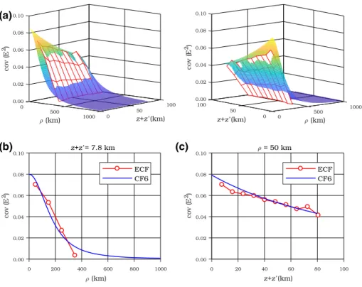
Our aim was to study the sensitivity of estimated parameters to the changes of GOCE satellite orbits and to other phenomena, which affect measured gradients (e.g. mass redistribution). We have followed the same strategy as described above. The Gaussian covariance model CF1 showing the best performance in the 1-dimensional case has been applied to this study. We have examined TZZ component of the disturbing gravitational tensor in all sub-regions. The radius of the approximation sphere remained unchanged (6628 km). ECF has been calculated from data collected in 6 two-month intervals during the year 2011. Parameters obtained by the least-squares method are listed in Table4. Value denoted ashis the mean altitude of GOCE satellite above GRS-80 reference ellipsoid in the particular sub-region. We assume that the variance will be increasing by decreasing altitude of GOCE orbit, and vice versa. This fact is clearly visible in Table4. Anomalous behavior occurs between time intervals of 07–08/2011, 09–10/2011 and 11–12/2011, especially in the sub-regions R1 and R2. However, the estimated parameters do not change dramatically within the particular sub-region. Disparity of variancesC0reaches a few mE2. This could be assigned mainly to satellite orbit changes. Therefore, the correct modeling of covariances requires consideration of different satellite altitudes above the approximation sphere and the tangent plane, respectively. However, the interpretation of this problem is not straightforward and further analyses would be required to formulate some clear conclusion.
Table 4 The estimated parameters of the covariance function CF1 (Gaussian) forTZZcomponent
Sub-reg. Param. 01–02 03–04 05–06 07–08 09–10 11–12 Mean
R1 C0(E2) 0.057 0.050 0.052 0.048 0.044 0.049 0.050
n(km) 220.8 207.9 203.1 208.3 207.2 208.6 209.3
h(km) 261.4 262.2 262.4 261.5 261.7 262.5 262.0
C0(E2) 0.404 0.384 0.383 0.378 0.405 0.377 0.388
R2 n(km) 221.5 216.4 218.5 214.5 221.2 215.9 218.0
h(km) 261.2 262.2 262.7 261.3 261.9 262.7 262.0
C0(E2) 0.023 0.021 0.021 0.022 0.023 0.022 0.022
R3 n(km) 148.6 146.9 145.6 146.7 148.6 148.2 147.4
h(km) 263.3 264.1 264.2 263.3 263.5 264.4 263.8
C0(E2) 0.029 0.028 0.027 0.028 0.027 0.026 0.027
R4 n(km) 227.2 228.5 225.3 229.1 228.6 226.2 227.5
h(km) 262.7 264.1 264.8 262.9 263.8 264.9 263.9
Numbers in the header row represent particular months of the year 2011
5 Experiment with the 2-dimensional local covariance functions
As stated previously, the evaluated 1-dimensional covariance function can take a different shape for various measurement cycles, even in the same region. The main reason is that the covariance function does not take into account the altitudes of data points above the spherical surface R1. Therefore, such model is not very suitable for SGG data. This disadvantage supersedes the 2-dimensional covariance function, which also enables spatial stochastic modeling.
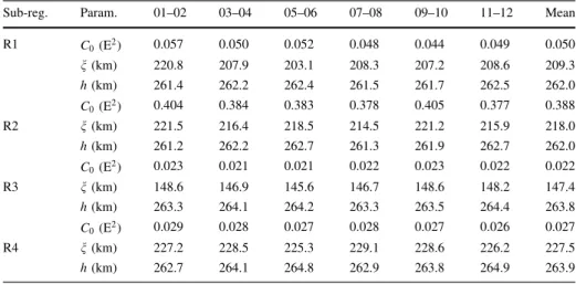
An analysis has been made in the same region of interest as depicted in Fig.2. Our goal was to examine stochastic dependencies of disturbing gravitational gradients in both the horizontal and the vertical direction. For this purpose, we have applied SGG data from the last measurement cycles collected from 1 June 2012 to 19 October 2013, when GOCE satellite has been stepwise decreasing its altitude. The radius of the approximation sphere of R1¼6595 km was chosen in such a way that all data points are situated above this sphere (z[0). In this case, both the planar distances q and the corresponding sum of altitudeszþz0were distributed into ten equally spaced bins. Figure4a shows ECF ofTZZ
component computed from Eq. (3) and corresponding to the sub-region R1 in two different views. It is possible to see a clear trend of covariance decreasing with increasing of both the planar distancesqand the sum of altitudeszþz0, as shown in Figure4b, c. Once again, only positive empirical covariances are displayed.
(a)
(b) (c)
Fig. 4 aTwo different views of the empirical covariance function ofTZZcomponent calculated in the sub- region R1 (red mesh) approximated by the 2-dimensional covariance model CF6 (coloured surface),b
0
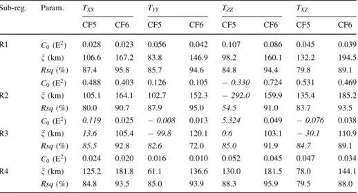
Empirical covariances were fitted by two analytical covariance models CF5 and CF6 described in Table2. Essential parameters, as variancesC0and correlation lengthsn, were estimated using the least-squares approach. Results are listed in Table5. Italic values indicate situations, where the least-squares estimates resulted in the improper values as the negative variances and the unrealistic correlation lengths. The analytical covariance function CF6 forTZZ component approximating empirical covariances is shown in Fig.4.
In compliance with the coefficient of determination, the analytical function CF6 accounts better performance. The highest variances are again typical for the sub-region R2 and the correlation lengths both for all evaluated components and the sub-regions vary between 103 and 195 km (only for CF6 model). This implies that covariance functions are highly responsive to the area of calculation and are, of course, different for particular components of disturbing gravitational tensor.
6 Interpolation of SGG data using least-squares collocation
The best way to demonstrate usefulness of the covariance function is to interpolate SGG data in order to produce regular local grid of disturbing gravitational gradients. For this purpose, the least-squares collocation (LSC) method has been used, where the covariance function plays an essential role. More details are explained e.g. in Moritz and Su¨nkel (1978), Moritz (1980).
Our experiment is restricted to the sub-region R1 and the largest component TZZ measured from 1 September 2013 to 19 October 2013. The regular grid with the resolution of 0:10:1 is located on the spherical surface with the radius ofR1¼6595 km. LSC enables to adjust both the trend of the disturbing gravitational gradients and the signal, which was modeled by the 2-dimensional covariance function CF6 with the estimated varianceC0¼0:086 E2and the correlation lengthn¼160:1 km (see Table5). We have considered the constant trend related to a systematic part of disturbing gravitational gra- dients in the tested sub-region and uncorrelated errors of observations corresponding to the
Table 5 The estimated parameters of local covariance models CF5 and CF6 (the 2-dimensional case)
Sub-reg. Param. TXX TYY TZZ TXZ
CF5 CF6 CF5 CF6 CF5 CF6 CF5 CF6
R1 C0(E2) 0.028 0.023 0.056 0.042 0.107 0.086 0.045 0.039
n(km) 106.6 167.2 83.8 146.9 98.2 160.1 132.2 194.5
Rsq(%) 87.4 95.8 85.7 94.6 84.8 94.4 79.8 89.1
C0(E2) 0.488 0.403 0.126 0.105 -0.330 0.724 0.531 0.469
R2 n(km) 105.1 164.1 102.7 152.3 -292.0 159.9 135.4 185.2
Rsq(%) 80.0 90.7 87.9 95.0 54.5 91.0 83.7 93.5
C0(E2) 0.119 0.025 -0.008 0.013 5.324 0.049 -0.076 0.038
R3 n(km) 13.6 105.4 -99.8 120.1 0.6 103.1 -30.1 110.9
Rsq(%) 85.5 92.8 82.6 72.0 85.0 91.9 84.7 89.1
C0(E2) 0.024 0.020 0.016 0.010 0.052 0.045 0.047 0.034
R4 n(km) 125.2 181.8 61.1 136.6 130.0 181.5 78.0 144.1
Rsq(%) 84.8 93.5 85.0 93.9 88.3 95.9 79.5 88.0
accuracy ofTZZcomponent given in EGG_TRF_2 products for SGG data. Figure5a shows directly interpolated disturbing gravitational gradientsTZZ in the sub-region R1 applying Delaunay triangulation method implemented in GMT 5 software (Wessel et al. 2013), which was used for producing figures. Using LSC, we have obtained smoothed disturbing gravitational gradients in Fig.5b interpolated in the regular grid with the given resolution and the suppressed random noise.
Proving the reliability of the local grid obtained by LSC, we have made the comparison with the corresponding set of grids produced by the Earth’s global gravity field models. We have used three recent models: TIM R5 up to d/o 200 (Brockmann et al.2014), EIGEN- 6C4 up to d/o 200 and 300 (Fo¨rste et al. 2014), and EGM2008 up to d/o 200 and 300 (Pavlis et al. 2012). TIM R5 is purely determined from the GOCE observations and is based on the time-wise approach. EIGEN-6C4 is a combined gravity field model using different satellite (LAGEOS, GRACE, and GOCE) and terrestrial data sets. EGM2008 was formed by combination of satellite, terrestrial, altimetry and airborne gravity data. Grids from these models were generated in ‘GrafLab’ software (Bucha and Jana´k2013) in the altitude corresponding to the radial distanceR1¼6595 km and with the same resolution as the produced LSC grid.
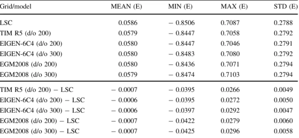
The basic summary statistics from the Earth’s global gravity field models are listed in Table6(upper part). For completeness, the residuals between model grids and the inter- polated LSC grid are presented. Residuals vary between0:043 E and 0.030 E with the mean close to zero, see the lower part of Table6. The best fit is obtained by applying EIGEN-6C4 model (d/o 300) with the standard deviation of 0.0047 E. It might indicate that there is still some useful signal in our solution corresponding to frequencies above d/o 200, and certain part of discrepancies is due to the omission error and noise. We recall that EIGEN-6C4 also includes GOCE data. The lowest agreement is evident for EGM2008 (d/o 200). However, discrepancies between compared models are negligible in most cases.
Let us look at the comparison with EIGEN-6C4 model (d/o 300) having the best fit more closely. Disturbing gravitational gradients obtained from this model are shown in Fig.6a and corresponding residuals in Fig. 6b. It is clearly visible that anomalous residuals mostly occur close to the limits of the sub-region R1. This effect is caused by missing information about the gravity field outside the sub-region, which has an influence on the covariance function construction and the interpolation procedure. Almost 99% of residuals
(a) (b)
Fig. 5 Disturbing gravitational gradientsTZZ: a directly interpolated from ‘measured’ gradients using
does not exceed the value of 0.01 E, what also confirms the centered histogram of residuals in Fig.6c. If we calculate the summary statistics of residuals from the restricted sub-region R1, which is reduced to/2h32N;38Niandk2h12E;18Ei, we will get more opti- mistic values: MEAN¼ 0:0006 E, MIN¼ 0:0125 E, MAX¼0:0102 E, and STD¼0:0037 E. In comparison with Table6, improvement of the standard deviation is more than 20%. This implies that a local grid should be created using a covariance function derived from an extended area, where more information about the surrounding Earth’s gravity field is included.
Table 6 The basic statistics of the Earth’s global gravity field models (upper part) and their comparison with LSC grid (lower part) in the sub-region R1 forTZZ component
Grid/model MEAN (E) MIN (E) MAX (E) STD (E)
LSC 0.0586 -0.8506 0.7087 0.2788
TIM R5 (d/o 200) 0.0579 -0.8447 0.7058 0.2792
EIGEN-6C4 (d/o 200) 0.0580 -0.8447 0.7046 0.2791
EIGEN-6C4 (d/o 300) 0.0580 -0.8483 0.7080 0.2792
EGM2008 (d/o 200) 0.0580 -0.8436 0.7071 0.2794
EGM2008 (d/o 300) 0.0579 -0.8474 0.7103 0.2794
TIM R5 (d/o 200)-LSC -0.0007 -0.0395 0.0266 0.0049
EIGEN-6C4 (d/o 200)-LSC -0.0006 -0.0395 0.0272 0.0050
EIGEN-6C4 (d/o 300)-LSC -0.0006 -0.0397 0.0292 0.0047
EGM2008 (d/o 200)-LSC -0.0007 -0.0422 0.0279 0.0060
EGM2008 (d/o 300)-LSC -0.0007 -0.0425 0.0296 0.0058
(a) (b) (c)
Fig. 6 Disturbing gravitational gradientsTZZ:afrom the Earth’s global gravity field model EIGEN-6C4 (up to d/o 300),bresiduals between EIGEN-6C4 model (up to d/o 300) and LSC grid, andcthe histogram of residuals
7 Conclusions
An analysis of local covariance functions of disturbing gravitational gradients derived from EGG_TRF_2 products was carried out in this study. Only covariance functions in the planar approximation were considered. Firstly, we have investigated four different types of the 1-dimensional covariance functions. In this situation, we assumed all data points are located on the approximation sphere, which is not exactly fulfilled for SGG data. The first numerical experiment reveals that the most appropriate from analytical covariance func- tions is the Gaussian function CF1 showing the best performance in all sub-regions. The parameters of the covariance function differ from region to region significantly. In our case of four adjacent sub-regions and TZZ component, the variance vary from 0.024 E2 to 0.412 E2 and the correlation length from 137 to 214 km. The lower correlation length indicates that the function is in average relatively more dissected. In addition, a time stability of essential parameters was studied. A sensitivity of estimated parameters to the changes of GOCE satellite orbit during various measurement cycles was showed. It appears that a correct modeling of stochastic dependencies between the observed gravity gradients requires evaluation of essential parameters directly from the region of interest. In general, the local covariance models with longer correlation length are more suitable for satellite gravity gradiometry data due to the smoothness of Earth’s gravity field.
Problem with the altitude variation of GOCE orbit can be treated by using the 2-di- mensional covariance function. Moreover, this enables us to perform the downward con- tinuation and the interpolation of measurements in one step. Presented procedure takes into account different altitudes of data points above the approximation sphere. We have studied two types of the 2-dimensional analytical functions. For all tested sub-regions, the covariance function CF6 shows better performance and numerical stability. Analysis showed again that estimated parameters are highly responsive to the input data in particular sub-region. The highest variances are typical for the sub-region R2 with the maximum signal amplitudes.
The 2-dimensional covariance model CF6 was applied to the interpolation of disturbing gravitational gradientsTZZinto the regular grid using the least-squares collocation method.
The local grid at the altitude corresponding to the radial distance ofR1¼6595 km was compared to values obtained from the recent Earth’s global gravity field models. We have used three recent models: TIM R5 up to d/o 200, EIGEN-6C4 up to d/o 200 and 300, and EGM2008 up to d/o 200 and 300. The best fit was achieved by applying EIGEN-6C4 model (d/o 300) with the mean of0:0006 E and the standard deviation of 0.0047 E. A cause of this may be the fact that this model also includes GOCE data. Disagreement of the interpolated grid with the model values mostly occurs near the limits of the sub-region, from which the covariance function was constructed. Omitting the 2 stripes around the limits of the sub-region brings improvement of the standard deviation of residuals more than 20%. The obtained results show practicability of the local covariance functions in planar approximation, ignoring the Earth’s sphericity, for solving the detail problems related to modeling of Earth’s gravity field using satellite gravity gradiometry data.
However, we must underline the fact that local grids computed following this approach are mostly intended for geophysical research and local applications.
Acknowledgements We gratefully acknowledge the reviewers comments and suggestions, which improved the paper essentially. This study is based on research carried out within the Slovak National Project VEGA 1/0954/15: Analysis of Global Data Sources and Possibilities of Their Application in the Refinement and Testing of Earth Gravity Field Models. Thanks also to the HPC center at the Slovak University of
Technology in Bratislava, which is a part of the Slovak Infrastructure of High Performance Computing (SIVVP project, ITMS code 26230120002, funded by the European region development funds, ERDF), for the computational time and resources made available.
References
Bouman J, Ebbing J, Fuchs M, Sebera J, Lieb V, Szwillus W, Haagmans R, Novak P (2016) Satellite gravity gradient grids for geophysics. Nat Sci Rep. doi:10.1038/srep21050
Brockmann JM, Zehentner N, Ho¨ck E, Pail R, Loth I, Mayer-Gu¨rr T, Schuh WD (2014) EGM_TIM_RL05:
an independent geoid with centimeter accuracy purely based on the GOCE mission. Geophys Res Lett 41:8089–8099. doi:10.1002/2014GL061904
Bucha B, Jana´k J (2013) A MATLAB-based graphical user interface program for computing functionals of the geopotential up to ultra-high degrees and orders. Comput Geosci 56:186–196
ESA (1999) Gravity field and steady-state ocean circulation mission, report for mission selection of the four candidate Earth explorer missions. Technical report ESA SP-1233(1), European Space Agency, ESA Publication Division
Fo¨rste C, Bruinsma S, Abrikosov O, Lemoine JM, Marty JC, Flechtner F, Balmino G, Barthelmes F, Biancale R (2014) EIGEN-6C4 the latest combined global gravity field model including GOCE data up to degree and order 2190 of GFZ Potsdam and GRGS Toulouse. doi:10.5880/icgem.2015.1. Accessed 12 Feb 2014
Gatti A, Migliaccio F, Reguzzoni M, Sanso` F (2013) Space-wise global grids of GOCE gravity gradients at satellite altitude. In: Geophysical research abstracts. Abstracts of the earth, planetary and space sci- ences, vol 15. Copernicus Publications, Go¨ttingen
Gruber T, Rummel R, Abrikosov O, Van Hess R (2010) GOCE level 2 product data handbook. Technical report GO-MA-HPF-GS-0110, The European GOCE Gravity Consortium EGG-C
Heiskanen WA, Moritz H (1967) Physical Geodesy. W. H, Freeman and Company, San Francisco Jekeli C (2010) Correlation modeling of the gravity field in classical geodesy. Springer, Berlin, pp 833–863.
doi:10.1007/978-3-642-01546-5_28
Moritz H (1980) Advanced physical geodesy. Wichmann, Karlsruhe
Moritz H, Su¨nkel H (1978) Approximation methods in geodesy. Wichmann, Karlsruhe
Pail R, Bruinsma S, Migliaccio F, Fo¨rste C, Goiginger H, Schuh WD, Ho¨ck E, Reguzzoni M, Brockmann JM, Abrikosov O, Veicherts M, Fecher T, Mayrhofer R, Krasbutter I, Sanso` F, Tscherning CC (2011) First GOCE gravity field models derived by three different approaches. J Geodesy 85:819–843. doi:10.
1007/s00190-011-0467-x
Pavlis NK, Holmes SA, Kenyon SC, Factor JK (2012) The development and evaluation of the earth gravitational model 2008 (EGM2008). J Geophys Res. doi:10.1029/2011JB008916
Rapp R (1978) Results of the application of least-squares collocation to selected geodetic problems. In:
Moritz H, Su¨nkel H (eds) Approximation methods in geodesy. Wichmann, Karlsruhe, pp 117–156 Rousseeuw PJ, Leroy AM (1987) Robust regression and outlier detection. Wiley, New York
Sˇprla´k M (2012) A graphical user interface application for evaluation of the gravitational tensor components generated by a level ellipsoid of revolution. Comput Geosci 46:77–83
Tscherning CC (1976) Covariance expressions for second and lower order derivatives of the anomalous potential. Technical report 225, Department of Geodetic Science, The Ohio State University Tscherning CC (2010) The use of least-squares collocation for the processing of GOCE data. Vermess
Geoinf 1:21–26
Wessel P, Smith WHF, Scharroo R, Luis J, Wobbe F (2013) Generic mapping tools: improved version released. Eos Trans Am Geophys Union 94(45):409–410. doi:10.1002/2013EO450001