Development and Experimental Validation of TRNSYS Simulation Model for Heat Wheel Operated in Air Handling Unit

(1)

energies

Article

Development and Experimental Validation of TRNSYS Simulation Model for Heat Wheel Operated in Air Handling Unit

Laith Al-Hyari and Miklos Kassai *

Department of Building Service Engineering and Process Engineering, Faculty of Mechanical Engineering, Budapest University of Technology and Economics, Muegyetem rkp. 3-9., H-1111 Budapest, Hungary;

alhyari@epget.bme.hu

* Correspondence: kas.miklos@gmail.com; Tel.:+36-20-362-8452

Received: 6 August 2020; Accepted: 16 September 2020; Published: 22 September 2020 Abstract: Reducing energy usage to save the environment is one of the main goals for the future.

The energy losses in ventilation have a huge impact on energy consumption in buildings. In this work, the energy performance of a heat recovery wheel system equipped in an air handling unit was tested year-round, and the results compared with the simulation output for the system using TRNSYS software. The selected conditioned space was the staffoffices of an H&M fashion shop, located in Eger, Hungary. Temperature, relative humidity, and air velocity sensors were placed at the wheel inlet and outlet sections to record data and determine the annual energy saving. The results revealed a good agreement between the measured and simulated results.

Keywords: building energy efficiency; air-to-air rotary heat exchanger; ventilation system; energy consumption

1. Introduction

Recently, concerns about building thermal load are receiving more attention as buildings are the most important energy consumers in most countries. Heat recovery is an approach for HVAC (Heating, Ventilation and Air Conditioning), which protects the environment and lowers the energy used in buildings. It improves energy efficiency and reduces energy consumption as the energy loss from ventilation reaches up to 50% of the total energy losses in buildings [1].

Various researchers carried out an energy-saving calculation using simulation. Often, the conventional approach cannot be performed under different ambient conditions. Energy-saving was investigated by several researchers, under different climate conditions [2,3]. Jani et al. [4] developed a TRNSYS (Transient System Simulation Tool) model to simulate a desiccant dehumidifier. Experimental measurements were obtained and compared to the simulation results. The simulated results showed that the system coefficient of performance had a critical influence when the regeneration temperature and relative humidity varied.

Improvement of the energy performance of a building using a heat pump was investigated by Wallin et al. [5]. The heat pump system was simulated using TRNSYS. They found that there is the potential to increase the heat exchange rate of the air-handling unit by coupling a heat pump to the system.

Zendehboudi et al. [6] determined the performance of a simple desiccant evaporative cooling cycle in four cities in Iran. The coefficient of performance (COP) was calculated in each case and the results were compared. They found that the city with the highest humidity levels had the best potential for the cooling system with the use of a desiccant wheel.

Based on the investigated literature, most of the case studies focused on the energy recovery system used in the ventilation system. Some of the research concentrated on an alternative hygroscopic

Energies2020,13, 4957; doi:10.3390/en13184957 www.mdpi.com/journal/energies

(2)

Energies2020,13, 4957 2 of 13

material for desiccant wheels to find the most energy-saving solution by using different composite materials [7]. Other studies focused on the energy performance of a building using TRNSYS simulation software to calculate the payback period when an energy recovery system was implemented [8].

Additionally, another study were performed on a run-around membrane energy exchanger (RAMEE) using simulation computed programs for various climates to estimate the reduced annual energy consumption and greenhouse gas emissions [9].

Different weather conditions, such as dry-bulb temperature, relative humidity, or airspeed, were used in the previous studies, and the effect of these parameters on the heating and cooling demands was investigated.

In this work, a complete system of an existing air handling unit (AHU) with an air-to-air rotary heat wheel was modeled for simulation using TRNSYS 18 [10]. The investigated running ventilation system was designed by the HVAC design engineer to supply fresh air and to provide the proper indoor air quality in the conditioned space, located in Eger, Hungary. The heating and cooling demands are covered by an independent system, the investigated ventilation system, which includes indoor air units connected to additional outdoor units and does not affect the ventilation energy consumption and was not investigated by our research work and investigations. The functioning hours of this retail location were between 7:00 a.m. and 8:00 p.m. A direct expansion coil integrated into the AHU was connected to a variable refrigerant volume (VRV) outdoor unit. The main objective and the novelty of this study was the development of a simulation model that was suitable for determining the energy consumption of ventilation systems and detailed investigation of the annual energy performance of the heat wheel with high accuracy. Temperature, humidity, and air velocity sensors were placed in selected sections in the air handling elements that significantly influence the heating and cooling processes.

The data measured from these sensors were recorded remotely using a monitoring system by a building management system (BMS) software. Simulated results were validated with the experimental data.

The effects of ambient parameters, such as regeneration temperature, dry bulb temperature, and relative humidity (RH), on energy performance was studied. The electrical energy consumption was calculated to obtain the energy-saving impact of the heat wheel on the VRV electric energy consumption.

2. Description of the Investigated AHU

The main air handling components of the investigated system were an air-to-air rotary heat wheel that recovered the sensible heat, a mixing box, supply fan, exhaust fan, and direct expansion cooling/heating (DX) coil connected to a variable refrigerant volume (VRV) outdoor unit. Figure1 shows the elements of the investigated AHU (Air Handling Unit) and describes the components.

Energies 2020, 13, x FOR PEER REVIEW 2 of 13

Based on the investigated literature, most of the case studies focused on the energy recovery system used in the ventilation system. Some of the research concentrated on an alternative hygroscopic material for desiccant wheels to find the most energy-saving solution by using different composite materials [7]. Other studies focused on the energy performance of a building using TRNSYS simulation software to calculate the payback period when an energy recovery system was implemented [8]. Additionally, another study were performed on a run-around membrane energy exchanger (RAMEE) using simulation computed programs for various climates to estimate the reduced annual energy consumption and greenhouse gas emissions [9].

Different weather conditions, such as dry-bulb temperature, relative humidity, or airspeed, were used in the previous studies, and the effect of these parameters on the heating and cooling demands was investigated.

In this work, a complete system of an existing air handling unit (AHU) with an air-to-air rotary heat wheel was modeled for simulation using TRNSYS 18 [10]. The investigated running ventilation system was designed by the HVAC design engineer to supply fresh air and to provide the proper indoor air quality in the conditioned space, located in Eger, Hungary. The heating and cooling demands are covered by an independent system, the investigated ventilation system, which includes indoor air units connected to additional outdoor units and does not affect the ventilation energy consumption and was not investigated by our research work and investigations. The functioning hours of this retail location were between 7:00 a.m. and 8:00 p.m. A direct expansion coil integrated into the AHU was connected to a variable refrigerant volume (VRV) outdoor unit. The main objective and the novelty of this study was the development of a simulation model that was suitable for determining the energy consumption of ventilation systems and detailed investigation of the annual energy performance of the heat wheel with high accuracy. Temperature, humidity, and air velocity sensors were placed in selected sections in the air handling elements that significantly influence the heating and cooling processes. The data measured from these sensors were recorded remotely using a monitoring system by a building management system (BMS) software. Simulated results were validated with the experimental data. The effects of ambient parameters, such as regeneration temperature, dry bulb temperature, and relative humidity (RH), on energy performance was studied.

The electrical energy consumption was calculated to obtain the energy-saving impact of the heat wheel on the VRV electric energy consumption.

2. Description of the Investigated AHU

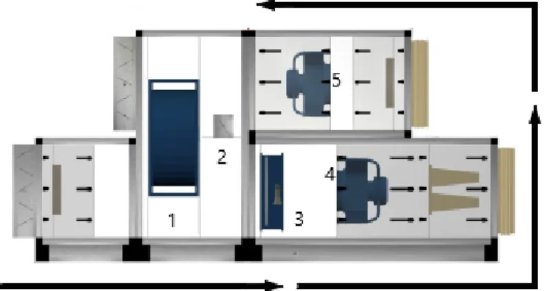
The main air handling components of the investigated system were an air-to-air rotary heat wheel that recovered the sensible heat, a mixing box, supply fan, exhaust fan, and direct expansion cooling/heating (DX) coil connected to a variable refrigerant volume (VRV) outdoor unit. Figure 1 shows the elements of the investigated AHU (Air Handling Unit) and describes the components.

Figure 1. The schematic arrangement of components of AHU with the heat wheel. 1: Air-to-air rotary heat wheel; 2: Mixing box; 3: Direct expansion cooling/heating (DX) coil; 4: Supply fan; 5: Exhaust fan.

Figure 1.The schematic arrangement of components of AHU with the heat wheel. 1: Air-to-air rotary heat wheel; 2: Mixing box; 3: Direct expansion cooling/heating (DX) coil; 4: Supply fan; 5: Exhaust fan.

The detailed configuration for the AHU following the path of the arrow around Figure1is as follows: the damper supply section, filter section, empty section, reciprocator heat wheel supply, mixing box supply, dx-coil, fan supply, filter supply, hole supply, hole return, filter return, and fan return.

(3)

The air damper was fully opened; the heat wheel rotation was operating at a constant speed throughout the experiment. The mixing box was fully closed so the supply air did not mix with the exhaust air.

The measurements were conducted from April 2019 to March 2020. The measurements were recorded on an hourly basis. The working hours of the retail shop were 7:00 a.m. to 8:00 p.m. throughout the year.

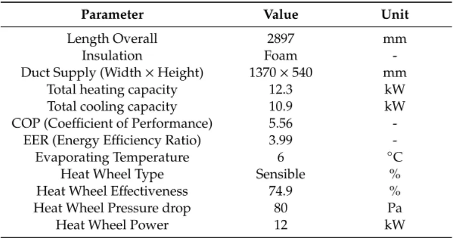
Figure2shows the air handling processes in the investigated AHU. The outside air passes through the air-to-air heat recovery wheel to recover the heat energy (state 1 to state 2) from the exhaust air inlet and it is further heated/cooled by a DX coil (state 2 to state 3) to the required supply air conditions at state 3. The air from the conditioned space enters the exhaust fan section and passes to the rotary heat wheel from the exhaust side, the supply air as upstream is passed through the rotary heat wheel, and it is cooled/heated from state 4 to state 5. On the regeneration side, the regeneration air is extracted (state 5 to state 6) into the ambient environment. The specification and the technical data of the AHU and the heat wheel, given by the producer, are provided in Table1. The technical data for the supply and return fan are presented in Table2. The technical specifications of the installed sensors and instrument are presented in Table3.

Figure 2. The schematic arrangement of components of AHU with the heat wheel.

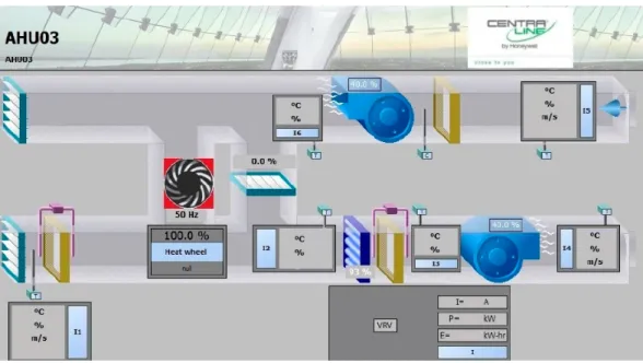
Experimental tests were conducted by measuring the temperature, relative humidity, mass flow rate across the AHU, process, and regeneration air stream flow rate simultaneously using sensors. A digital sensor was used for precise measurement of the temperature and relative humidity at different states in AHU. The regeneration airflow rate at different sections in the AHU was also measured with the digital sensors. A digital temperature controller in a conditioned space controls the temperature depending on the changes in room temperature. The computer software by the manufacturer for monitoring and recording was used to observe and record all the data obtained by the sensors in the AHU. Since this research focused on the annual heat recovering by the heat wheel, the mixing box between the inlet and outlet sections of the AHU was set to be closed during the investigations. Figure 3 shows a screenshot of the investigated AHU in the building management system(BMS) program.

The recorded data were evaluated. Energetic investigations were performed on the performance of AHU using the measurements. To achieve this, the mathematical approaches described in Section 3 were implemented.

Figure 3. The AHU schematic in the building management system (BMS).

3. Description of the Used Mathematical Model

In this study, the performance of the air handling unit was investigated by calculating the cooling/heating capacity of the direct expansion coil, electrical power input of the VRV, coefficient of

Figure 2.The schematic arrangement of components of AHU with the heat wheel.

Table 1.Specification and technical data for AHU and energy wheel.

Parameter Value Unit

Length Overall 2897 mm

Insulation Foam -

Duct Supply (Width×Height) 1370×540 mm

Total heating capacity 12.3 kW

Total cooling capacity 10.9 kW

COP (Coefficient of Performance) 5.56 -

EER (Energy Efficiency Ratio) 3.99 -

Evaporating Temperature 6 ^◦C

Heat Wheel Type Sensible %

Heat Wheel Effectiveness 74.9 %

Heat Wheel Pressure drop 80 Pa

Heat Wheel Power 12 kW

(4)

Energies2020,13, 4957 4 of 13

Table 2.Technical data for the supply and return fan.

Device Parameter Value Unit

Supply Fan Type Centrifugal Fan -

Total Static Pressure 619 Pa

Flow Design 2250 m³/h

Rated Power 0.7 kW

Return Fan Type Centrifugal Fan -

Total Static Pressure 473 pa

Flow Design 1850 m³/h

Rated Power 0.49 kW

Table 3.Specifications of the sensors and instruments.

Device Working Range Accuracy

Temperature Sensor −40 to 150^◦C ±0.4^◦C

Humidity Sensor 10–90% ±3%

Air velocity Sensor 2–20 m/s ±0.2 m/s

Electricity energy meter 5–100 A ±1%

Experimental tests were conducted by measuring the temperature, relative humidity, mass flow rate across the AHU, process, and regeneration air stream flow rate simultaneously using sensors.

A digital sensor was used for precise measurement of the temperature and relative humidity at different states in AHU. The regeneration airflow rate at different sections in the AHU was also measured with the digital sensors. A digital temperature controller in a conditioned space controls the temperature depending on the changes in room temperature. The computer software by the manufacturer for monitoring and recording was used to observe and record all the data obtained by the sensors in the AHU. Since this research focused on the annual heat recovering by the heat wheel, the mixing box between the inlet and outlet sections of the AHU was set to be closed during the investigations. Figure3 shows a screenshot of the investigated AHU in the building management system (BMS) program.

The recorded data were evaluated. Energetic investigations were performed on the performance of AHU using the measurements. To achieve this, the mathematical approaches described in Section3 were implemented.

Figure 2. The schematic arrangement of components of AHU with the heat wheel.

Experimental tests were conducted by measuring the temperature, relative humidity, mass flow rate across the AHU, process, and regeneration air stream flow rate simultaneously using sensors. A digital sensor was used for precise measurement of the temperature and relative humidity at different states in AHU. The regeneration airflow rate at different sections in the AHU was also measured with the digital sensors. A digital temperature controller in a conditioned space controls the temperature depending on the changes in room temperature. The computer software by the manufacturer for monitoring and recording was used to observe and record all the data obtained by the sensors in the AHU. Since this research focused on the annual heat recovering by the heat wheel, the mixing box between the inlet and outlet sections of the AHU was set to be closed during the investigations. Figure 3 shows a screenshot of the investigated AHU in the building management system(BMS) program.

The recorded data were evaluated. Energetic investigations were performed on the performance of AHU using the measurements. To achieve this, the mathematical approaches described in Section 3 were implemented.

Figure 3. The AHU schematic in the building management system (BMS).

In this study, the performance of the air handling unit was investigated by calculating the cooling/heating capacity of the direct expansion coil, electrical power input of the VRV, coefficient of

Figure 3.The AHU schematic in the building management system (BMS).

(5)

In this study, the performance of the air handling unit was investigated by calculating the cooling/heating capacity of the direct expansion coil, electrical power input of the VRV, coefficient of performance (COP), and the effectiveness of the heat recovery wheel. The cooling/heating capacity (Q^._c) of the system is expressed in Equation (1) [11]:

.

Q_c=m^.a(h3−h2) (1) wherem^.ais the mass flow rate of air leaving the coil (kg/s), which is calculated by the multiplication of the average measured velocity of the air (m/s) and the area of the cross-section of air duct (0.74 m²), and the density of the air(_ρ_air), which is around 1.2 kg/m³.h₂andh₃are the enthalpies of the air in states 2 and 3, respectively (Figure2).

The power consumption of the VRV systemEcomp[12] is calculated using Equation (2):

Et=Ecomp (2)

whereEcompis the power consumption of the compressor, which is measured by using an energy meter.

.

Q_r is the regeneration heat supplied by the energy wheel [11], which is calculated by:

.

Q_r=_m^._r(_h₁⁻_h₂) ₍₃₎ wherem^.r is the mass flow rate of regeneration air and h1and h2are the enthalpies in states 1 and 2, respectively.

The coefficient of performance (COP) of the system is calculated [13] using the Equation (4):

COP=

.

Q_c

Et (4)

The sensible effectiveness of heat recovery wheel (HRW) is determined by Equation (5) [14]:

ε=

V.s(T₁−T2)

V._min(T₁−T₄) ⁽⁵⁾ whereT₁is the outdoor air temperature at the supply inlet of the heat wheel,T₂is the air temperature in the supply outlet of the heat wheel, andT₄is the air temperature in the exhaust inlet of the heat wheel.V^.sis the volume flow rate of the supply air (m³/h) andV^._minis the smaller volume flow rate (supply or exhaust air) (m³/h).

The sensible heat transfer is determined by Equation (6) [15]:

.

Q_s=V^.min·ρair·Cp·(T1−T4). (6) 4. Description of the Developed TRNSYS Simulation Model

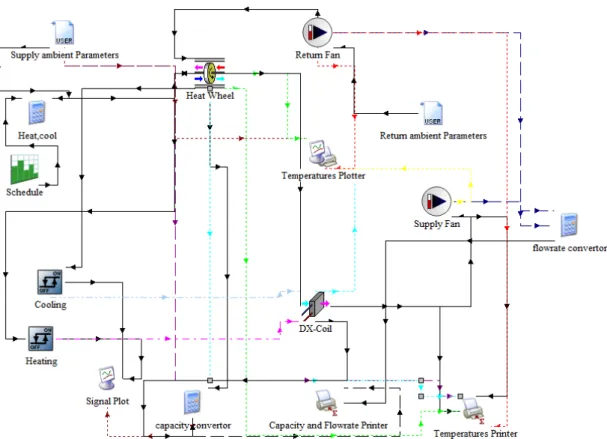
Figure4shows the TRNSYS model of the AHU system. The components used in the model were selected from the TRNSYS TESS library. The system was modeled and simulated using TRNSYS to compare the performance of the simulated and the measured data throughout the year.

(6)

Energies2020,13, 4957 6 of 13

Figure 4. TRNSYS simulation model.

5. Model Validation

The new TRNSYS model was validated by comparing this model with the actual data [16].

Measured weather parameters were used as input data for the simulation models. Then a comparison was conducted between the simulated and measured values to determine the accuracy of the developed TRNSYS model. As hourly data analysis was used, the criteria of normalized mean bias error (NMBE) and coefficient of variation of the root mean square error (CVRMSE) were 10% and 30%, respectively. NMBE and CVRMSE are calculated by Equations (6) and (7), respectively, where 𝑦 is the measured value, 𝑦 is the predicted or simulated value, 𝑦 is the mean of the 𝑦 values, and N is the total number of measured points [17].

𝑁𝑀𝐵𝐸 =

𝑁 ∑ (𝑦 − 𝑦 )1

𝑦 · 100 (7)

𝐶𝑉(𝑅𝑀𝑆𝐸) =

𝑁 ∑ (𝑦 − 𝑦 )1

𝑦 . 100 (8)

6. Results and Discussion

The measured and simulated ambient temperature from the TRNSYS model during winter and summer are presented in this section. The functioning hours of the AHU were between 7:00 a.m. and 8:00 p.m., which means the unit was turned off after 8:00 p.m.

Figure 5 shows a graph representing the fresh outlet from the heat wheel and exhaust inlet between the simulated and measured temperature the summer period (cooling) Figure 6 represents the fresh outlet from the heat wheel and exhaust inlet between the simulated and measured temperature in the winter period (heating).

Figure 4.TRNSYS simulation model.

Type 9e (data reader) was used to read the ambient parameters for the measured outdoor dry bulb temperature and relative humidity. These parameters were read from an external file that contained the measured outdoor ambient parameters. The same type was used to read the return ambient parameters and the volume flow rate from the indoor space. The actual measurements from the outdoor and the return from the space were used to perform an accurate validation of the TRNSYS model.

The rotary heat wheel was modeled as type 760 as it represents sensible air-to-air heat recovery with controlled outlet conditions, DX coil was modeled as type 136, type 65c, and type 46a used as an output plotter and printer. Type 111b represented the supply and return air fans. The cooling and heating process signals were monitored using type 165 from the TESS library. Type 14 (time-dependent function) was used as a schedule for the running system to work during the working hours (7:00 a.m.

to 8:00 p.m.).

5. Model Validation

The new TRNSYS model was validated by comparing this model with the actual data [16].

Measured weather parameters were used as input data for the simulation models. Then a comparison was conducted between the simulated and measured values to determine the accuracy of the developed TRNSYS model. As hourly data analysis was used, the criteria of normalized mean bias error (NMBE) and coefficient of variation of the root mean square error (CVRMSE) were 10% and 30%, respectively.

NMBE and CVRMSE are calculated by Equations (6) and (7), respectively, whereyiis the measured value, ˆyiis the predicted or simulated value,yis the mean of theyivalues, and N is the total number of measured points [17].

NMBE=

1 N

PN

i (y_i−y^ˆ_i)

y ·100 (7)

(7)

CV(RMSE) = r

1 N

P_N

i (yi−y^ˆ_i)

2

y .100 (8)

6. Results and Discussion

The measured and simulated ambient temperature from the TRNSYS model during winter and summer are presented in this section. The functioning hours of the AHU were between 7:00 a.m. and 8:00 p.m., which means the unit was turned offafter 8:00 p.m.

Figure5shows a graph representing the fresh outlet from the heat wheel and exhaust inlet between the simulated and measured temperature the summer period (cooling) Figure6represents the fresh outlet from the heat wheel and exhaust inlet between the simulated and measured temperature in the winter period (heating).Energies 2020, 13, x FOR PEER REVIEW 7 of 13

Figure 5. The fresh outlet and exhaust inlet around the heat during summer.

Figure 6. The fresh outlet and exhaust inlet around the heat during winter.

On the heat wheel recovery sides, the monitored fresh air outlet from the heat wheel during summer was slightly higher than the simulation results, which would lead to higher energy consumption in the DX coil. During winter, it had lower values, which would lead to more energy from the VRF outdoor unit being consumed.

In the exhaust inlet section of the heat wheel, temperatures with a slight difference in the measured values temperature were observed during both winter and summer months.

In the following equations, the supply and exhaust air volume flow rate (during summer and winter) will be calculated.

For summer, the fresh air volume flow supply was measured by a sensor located at state 1. The mathematical approach to calculate the air volume flow rate is:

𝑉 = A · ω · 3600 (9)

where 𝑉 is the volume flow rate of the supply air (m³/h), A is the area of cross-section of air duct (0.74 m²), and ω is the average velocity of the supply fresh air in summer (0.411 m/s).

𝑉 = 1095 (m /h)

The exhaust fresh air volume flow was measured by a sensor located at state 5. The average velocity of the exhaust fresh air in summer was 0.339 m/s.

𝑉 = 901.5 (m /h)

Figure 5.The fresh outlet and exhaust inlet around the heat during summer.

Figure 5. The fresh outlet and exhaust inlet around the heat during summer.

Figure 6. The fresh outlet and exhaust inlet around the heat during winter.

For summer, the fresh air volume flow supply was measured by a sensor located at state 1. The mathematical approach to calculate the air volume flow rate is:

𝑉 = A · ω · 3600 (9)

where 𝑉 is the volume flow rate of the supply air (m³/h), A is the area of cross-section of air duct (0.74 m²), and ω is the average velocity of the supply fresh air in summer (0.411 m/s).

𝑉 = 1095 (m /h)

𝑉 = 901.5 (m /h)

Figure 6.The fresh outlet and exhaust inlet around the heat during winter.

(8)

Energies2020,13, 4957 8 of 13

For summer, the fresh air volume flow supply was measured by a sensor located at state 1.

The mathematical approach to calculate the air volume flow rate is:

.

Vs=A·ω_avg·3600 (9)

whereV^.sis the volume flow rate of the supply air (m³/h), A is the area of cross-section of air duct (0.74 m²), andω_avgis the average velocity of the supply fresh air in summer (0.411 m/s).

.

Vss=1095(m³/h)

.

Ves=901.5(m³/h)

For winter, the average velocity of the supply fresh air was 0.362 m/s.

.

Vsw=963(m³/h)

The average velocity of the exhaust fresh air in winter was 0.268 m/s.

.

Vew=714.3(m³/h)

The reason for some differences in the higher supply airflow is that exhaust airflow is only an operational set since there are many doors and windows in the building that have leakages, so some of the supply air leaves the conditioned spaces as it is injected by the diffusers. The simulation volume flow rate values were taken from the monitored values as these values were inputs in the TRNSYS simulation.

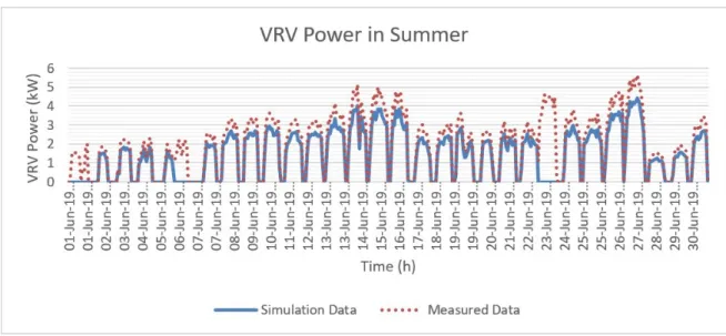
Figures7and8represent the VRV power (in kW) for summer and winter, respectively.

𝑉 = 963 (m /h)

𝑉 = 714.3 (m /h)

Figures 7 and 8 represent the VRV power (in kW) for summer and winter, respectively.

Figure 7. The measured and simulated power consumption in summer.

Figure 8. The measured and simulated power consumption in winter.

Figures 7 and 8 show that the monitored VRV power in summer was higher than the simulated results. This could be due to the high monitored ambient temperatures during June. The results of the VRV power in winter showed values between the measured and simulated results.

Figures 9 and 10 show the sensible effectiveness values (

ɛ

s) of the heat wheel as a function of fresh air inlet temperature in winter (heating) and summer (cooling), respectively.

Figure 7.The measured and simulated power consumption in summer.

(9)

Energies2020,13, 4957 9 of 13

𝑉 = 963 (m /h)

𝑉 = 714.3 (m /h)

Figures 7 and 8 represent the VRV power (in kW) for summer and winter, respectively.

Figure 7. The measured and simulated power consumption in summer.

Figure 8. The measured and simulated power consumption in winter.

Figures 7 and 8 show that the monitored VRV power in summer was higher than the simulated results. This could be due to the high monitored ambient temperatures during June. The results of the VRV power in winter showed values between the measured and simulated results.

Figures 9 and 10 show the sensible effectiveness values (

ɛ

^s) of the heat wheel as a function of fresh air inlet temperature in winter (heating) and summer (cooling), respectively.

Figure 8.The measured and simulated power consumption in winter.

Figures7and8show that the monitored VRV power in summer was higher than the simulated results. This could be due to the high monitored ambient temperatures during June. The results of the VRV power in winter showed values between the measured and simulated results.

Figures9and10show the sensible effectiveness values (εs) of the heat wheel as a function of fresh air inlet temperature in winter (heating) and summer (cooling), respectively.

Figure 9. The measured and simulated sensible effectiveness values in summer.

Figure 10. The measured and simulated sensible effectiveness values in winter.

Figure 10 shows that the measured effectiveness in winter varied with an average of 74.1%. The simulation had an almost constant trend throughout the month, with an average value of around 73.9%. Figure 9 shows that the measured effectiveness of the HWR in summer had relatively higher values than the simulated results. The maximum value reported was around 97.6%, with an average effectiveness of around 80.2%. The simulation results showed more stable values of effectiveness than the measured values as a function of outdoor air temperature.

The difference in effectiveness between the measured and simulated values occurred due to the heat wheel in the simulation that takes the value of effectiveness as an input value. That is why it showed almost constant value throughout the month. The effectiveness value for the heat wheel was calculated according to Equation (5) depending on the measured temperatures recorded.

Figure 11 shows the sensible heat transfer (kWh) by the heat wheel. It represents the heat transfer rate for the whole year by heat wheel.

Figure 9.The measured and simulated sensible effectiveness values in summer.

Figure10shows that the measured effectiveness in winter varied with an average of 74.1%.

The simulation had an almost constant trend throughout the month, with an average value of around 73.9%. Figure9shows that the measured effectiveness of the HWR in summer had relatively higher values than the simulated results. The maximum value reported was around 97.6%, with an average effectiveness of around 80.2%. The simulation results showed more stable values of effectiveness than the measured values as a function of outdoor air temperature.

(10)

Energies2020,13, 4957 10 of 13

Figure 9. The measured and simulated sensible effectiveness values in summer.

Figure 10. The measured and simulated sensible effectiveness values in winter.

Figure 10 shows that the measured effectiveness in winter varied with an average of 74.1%. The simulation had an almost constant trend throughout the month, with an average value of around 73.9%. Figure 9 shows that the measured effectiveness of the HWR in summer had relatively higher values than the simulated results. The maximum value reported was around 97.6%, with an average effectiveness of around 80.2%. The simulation results showed more stable values of effectiveness than the measured values as a function of outdoor air temperature.

Figure 11 shows the sensible heat transfer (kWh) by the heat wheel. It represents the heat transfer rate for the whole year by heat wheel.

Figure 10.The measured and simulated sensible effectiveness values in winter.

Figure11shows the sensible heat transfer (kWh) by the heat wheel. It represents the heat transfer rate for the whole year by heat wheel.Energies 2020, 13, x FOR PEER REVIEW 10 of 13

Figure 11. The measured and simulated sensible heat transfer (kWh).

The calculated sensible heat transfer by the measured parameters of the heat wheel was relatively higher than the simulation results for many reasons, such as the higher calculated effectiveness from the measured ambient parameters and the higher difference between the supply inlet and the exhaust inlet temperature in the measured values.

Figure 12 shows the accumulated electrical energy consumption in kWh for the VRF outdoor unit throughout the year in the winter season (heating) and summer season (cooling).

Figure 12. The measured and simulated electrical energy consumption in winter and summer (heating and cooling).

Figure 12 shows good agreement between the measured and simulated results in hourly energy use. The simulated energy uses in heating and cooling mode were all within the range of ±10% (Table 4). This is within the acceptable criteria range, with the model considered calibrated if the absolute value of NMBE was less than 10%. The CVRMSE values for heating and cooling mode were 19% and 24%, respectively, which are considered acceptable as the criterion for CVRMSE is less than 30%

based on ASHREA Guideline 14-2014[18]. Table 4. Shows the calibration results of the simulation model.

Figure 11.The measured and simulated sensible heat transfer (kWh).

Figure12shows the accumulated electrical energy consumption in kWh for the VRF outdoor unit throughout the year in the winter season (heating) and summer season (cooling).

(11)

Energies2020,13, 4957 11 of 13 Figure 11. The measured and simulated sensible heat transfer (kWh).

Figure 12 shows the accumulated electrical energy consumption in kWh for the VRF outdoor unit throughout the year in the winter season (heating) and summer season (cooling).

Figure 12. The measured and simulated electrical energy consumption in winter and summer (heating and cooling).

Figure 12 shows good agreement between the measured and simulated results in hourly energy use. The simulated energy uses in heating and cooling mode were all within the range of ±10% (Table 4). This is within the acceptable criteria range, with the model considered calibrated if the absolute value of NMBE was less than 10%. The CVRMSE values for heating and cooling mode were 19% and 24%, respectively, which are considered acceptable as the criterion for CVRMSE is less than 30%

based on ASHREA Guideline 14-2014[18]. Table 4. Shows the calibration results of the simulation model.

Figure 12.The measured and simulated electrical energy consumption in winter and summer (heating and cooling).

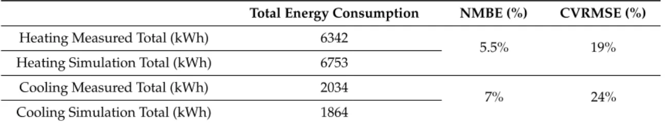
Figure12shows good agreement between the measured and simulated results in hourly energy use. The simulated energy uses in heating and cooling mode were all within the range of±10% (Table4).

This is within the acceptable criteria range, with the model considered calibrated if the absolute value of NMBE was less than 10%. The CVRMSE values for heating and cooling mode were 19% and 24%, respectively, which are considered acceptable as the criterion for CVRMSE is less than 30% based on ASHREA Guideline 14-2014 [18]. Table4. Shows the calibration results of the simulation model.

Table 4.Calibration results of the simulation model.

Total Energy Consumption NMBE (%) CVRMSE (%)

Heating Measured Total (kWh) 6342

5.5% 19%

Heating Simulation Total (kWh) 6753

Cooling Measured Total (kWh) 2034

7% 24%

Cooling Simulation Total (kWh) 1864

7. Conclusions

The simulated results of the AHU air-conditioning system emphasize the good performance of the system. The main findings of this research study are summarized as follows:

(1) The analysis of the supply air condition (fresh air inlet) of the heat wheel showed that the system can save energy in different weather conditions and it is more useful than the conventional air conditioning systems.

(2) The change in the fresh inlet temperature air has a major influence on the system performance.

The performance of the AHU air-conditioning system can be further enhanced by equipping a sorption wheel for the supply of regeneration energy to maximize the energy savings by transfer of the humidity air from the extract air.

(3) The sensible effectiveness values of the heat wheel measured were higher than the simulated data in summer, whereas it was lower in winter.

(4) The simulation value of sensible effectiveness showed a constant trend that was close to the given effectiveness values in the technical data sheet of the producer (74.9%).

(5) The NMBE and CVRMSE used to validate the model showed that the TRNSYS model has an acceptable range as the criteria for NMBE and CVRMSE are less than 10% and 30%, respectively. The developed TRNSYS model can be useful for predicting the performance of such extreme conditions.

(12)

Energies2020,13, 4957 12 of 13

Altogether, the heat wheel was found to be reliable in performance, environmentally friendly, and has a notable energy-saving impact on the electrical consumption. The developed TRNSYS model can be used to simulate the performance heat wheel under different operating conditions.

Author Contributions: M.K. provided funding for the research, developed the measurement system, and conducted the field study for the topic. The simulation model was developed and validated using the measured results by L.A.-H. and supervised by M.K. The text was written by L.A.-H. and amended by M.K.

All authors have read and agreed to the published version of the manuscript.

Funding:The sensors, instruments, and transducers were financially supported and installed, as well as BMS software for data recording was constructed for this research work, by the national Intherm Ltd. This research project was financially supported by the National Research, Development and Innovation Office from NRDI Fund (grant number: NKFIH PD_18 127907) and János Bolyai Research Scholarship of the Hungarian Academy of Sciences, Budapest, Hungary. The research reported in this paper and carried out at the Budapest University of Technology and Economics was supported by the TKP2020, National Challenges Program of the National Research Development and Innovation Office (BME NC TKP2020), as well as by the Higher Education Excellence Program of the Ministry of Human Capacities in the frame of Artificial Intelligence research area of Budapest University of Technology and Economics (BME FIKP-MI). The authors acknowledge the Hungary Government for their financial support as the Stipendium Hungaricum Scholarship.

Acknowledgments: The author wishes to thankÁrpád Nagy and Gyula Szabófrom the Intherm Ltd. group, as well as Balázs Zuggóand Noémi Bálint from the Daikin Hungary Ltd. group for providing the research background with their professional, technical, and practical knowledge for this research.

Conflicts of Interest:The authors declare no conflict of interest.

Nomenclature

Abbreviations

h Enthalpy (kJ/kg)

m. Air mass flow rate (kg/h)

RH Relative Humidity (%)

Q Heat Capacity (kW)

Et Power Consumption (kW)

T Temperature (^◦C)

.

V Air volume flow rate (m³/h)

VRV Variable Refrigerant Flow

AHU Air Handling Unit

HWR Heat Wheel Recovery

COP Coefficient of Performance

Greek Letters

ε effectiveness

τ time (h)

ρair Density of the air (kg/m³)

Cp Specific heat capacity (kJ/kg^◦C)

Subscripts

Ei Exhaust air inlet

o Outdoor

Si Supply air inlet

So Supply air outlet

ss supply air in summer

es exhaust air in summer

sw supply air in winter

ew exhaust air in winter

s Sensible

(13)

References

1. Kassai, M.; Al-Hyari, L. Experimental investigation on operation parameters of 3Å molecular sieve desiccant coated total energy recovery wheel for maximum effectiveness.Therm. Sci.2020,24, 2113–2124. [CrossRef]

2. Wan, K.K.W.; Li, D.H.W.; Liu, D.; Lam, J.C. Future trends of building heating and cooling loads and energy consumption in different climates.Build. Environ.2011,46, 223–234. [CrossRef]

3. Ahmed, K.; Carlier, M.; Feldmann, C.; Kurnitski, J. A New Method for Contrasting Energy Performance and Near-Zero Energy Building Requirements in Different Climates and Countries.Energies2018,11, 1334.

[CrossRef]

4. Jani, D.B.; Mishra, M.; Sahoo, P.K. Performance studies of hybrid solid desiccant - vapor compression air-conditioning system for hot and humid climates.Energy Build.2015,102, 284–292. [CrossRef]

5. Jörgen, W.; Joachim, C. Improving heat recovery using retrofitted heat pump in air handling unit with energy wheel.Appl. Therm. Eng.2014,64, 823–829.

6. Zendehboudi, A.; Hashemi, R. A Study on the Performance of a Solar Desiccant Cooling System by TRNSYS in Warm and Humid Climatic Zone of IRAN.Int. J. Adv. Sci. Technol.2014,69, 13–18. [CrossRef]

7. Bareschino, P.; Pepe, F.; Roselli, C.; Sasso, M.; Tariello, F. Desiccant-based air handling unit alternatively equipped with three hygroscopic materials and driven by solar energy.Energies2019,12, 1543. [CrossRef]

8. Rasouli, M.; Simonson, C.J.; Besant, R.W. Applicability and optimum control strategy of energy recovery ventilators in different climatic conditions.Energy Build.2010,42, 1376–1385. [CrossRef]

9. Rasouli, M.; Akbari, S.; Simonson, C.J.; Besant, R.W. Energetic, economic and environmental analysis of a health-care facility HVAC system equipped with a run-around membrane energy exchanger.Energy Build.

2014,69, 112–121. [CrossRef]

10. TRNSYS. Trnsys 17—Input—Output—Parameter Reference, A Transient System Simulation Program User’s Manual. Solar Energy Laboratory, University of Wisconsin, Madison, 2011. Available online:

http://web.mit.edu/parmstr/Public/TRNSYS/04-MathematicalReference.pdf(accessed on 18 September 2020).

11. Speerforck, A.; Schmitz, G. Experimental investigation of a ground-coupled desiccant assisted air conditioning system.Appl. Energy2016,181, 575–585. [CrossRef]

12. Jani, D.B.; Mishra, M.; Sahoo, P.K. Performance analysis of a solid desiccant assisted hybrid space cooling system using TRNSYS.J. Build. Eng.2018,19, 26–35. [CrossRef]

13. De Antonellis, S.; Intini, M.; Joppolo, C.M.; Leone, C. Design Optimization of Heat Wheels for Energy Recovery in HVAC Systems.Energies2014,7, 7348–7367. [CrossRef]

14. Kassai, M. Energy Performance Investigation of a Direct Expansion Ventilation Cooling System with a Heat Wheel. Energies2019,12, 4267. [CrossRef]

15. ASHRAE Standard. Standard 84-1991, Method of Testing Air-to-Air Heat Exchangers; American Society of Heating, Refrigerating and Air Conditioning, Engineers Inc.: Atlanta, GA, USA, 1991.

16. Hong, T.; Sun, K.; Zhang, R.; Hinokuma, R.; Kasahara, S.; Yura, Y. Development and validation of a new variable refrigerant flow system model in EnergyPlus.Energy Build.2016,117, 399–411. [CrossRef]

17. Granderson, J.; Touzani, S.; Custodio, C.; Sohn, M.; Fernandes, S.Assessment of Automated Measurement and Verification (M&V) Methods; Building Technology and Urban Systems Division, Lawrence Berkeley National Laboratory: Berkeley, CA, USA, 2015.

18. American Society of Heating, Ventilating, and Air Conditioning Engineers (ASHRAE).Guideline 14-2014, Measurement of Energy and Demand Savings; Technical Report; American Society of Heating, Ventilating, and Air Conditioning Engineers: Atlanta, GA, USA, 2014.

©2020 by the authors. Licensee MDPI, Basel, Switzerland. This article is an open access article distributed under the terms and conditions of the Creative Commons Attribution (CC BY) license (http://creativecommons.org/licenses/by/4.0/).