Homoclinic solutions of singular differential equations with φ-Laplacian

Homoclinic solutions of singular differential equations with φ-Laplacian

Lukáš Rach ˚unek

and Irena Rach ˚unková

1Department of Algebra and Geometry, Faculty of Science, Palacký University Olomouc, 17. listopadu 12, 771 46 Olomouc, Czech Republic

2Department of Mathematical Analysis and Applications of Mathematics, Faculty of Science, Palacký University Olomouc, 17. listopadu 12, 771 46 Olomouc, Czech Republic

Received 8 March 2018, appeared 28 August 2018 Communicated by Josef Diblík

Abstract. A singular nonlinear initial value problem (IVP) with a φ-Laplacian of the form

(p(t)φ(u⁰(t)))⁰+p(t)f(φ(u(t))) =_0, u(₀) =u₀∈[L₀, 0)_, u⁰(₀) =₀

is investigated on the half-line[0,∞). Here, functionφis smooth and increasing onR withφ(0) =0, function f is locally Lipschitz continuous with three zerosφ(L0)<0<

φ(L), function pis smooth and increasing on(0,∞), and the problem is singular in the sense that p(0) =0 and 1/p(t)may not be integrable on [0, 1]. The main result of the paper is the existence of homoclinic solutions defined as nondecreasing solutionsuof the IVP satisfying limt→∞u(t) =L.

Keywords: second order ODE, time singularity,φ-Laplacian, homoclinic solution, half- line.

2010 Mathematics Subject Classification: 34A12, 34C37, 34D05.

1 Introduction

We investigate solutions of the initial value problem (IVP)

(p(t)φ(u⁰(t)))⁰+p(t)f(φ(u(t))) =0, t∈ (0,∞), (1.1) u(0) =u₀, u⁰(0) =0, u₀∈[L₀, 0), (1.2) where

φ∈C¹(_R), φ⁰(x)>0 forx∈(_R\ {0}), (1.3)

φ(_R) =_R, φ(0) =0, (1.4)

L₀<0< L, f(φ(L₀)) = f(0) = f(φ(L)) =0, (1.5) f ∈Lip[φ(L0),φ(L)], x f(x)>0 forx∈((φ(L0),φ(L))\ {0}), (1.6) p∈C[0,∞)∩C¹(0,∞), p⁰(t)>0 fort ∈(0,∞), p(0) =0. (1.7)

In particular, we find additional conditions for p, φ and f which guarantee for some u₀ ∈ [L0, 0)the existence of a nondecreasing solution of IVP (1.1), (1.2) converging toL fort→ _∞.

Note that if we extend the function p in equation (1.1) from the half-line onto R as an even function and assume thatφis odd, then any solutionuof IVP (1.1), (1.2) with lim_t→_∞u(t) = L fulfils limt→−_∞u(t) = L. Such solution u is called a homoclinic solution. This is a motivation for Definition1.4. Due to condition (1.7) the function 1/p(t) may not be integrable on [0, 1] and consequently equation (1.1) has a time singularity at t = 0. Problems of this type arise in hydrodynamics [10] or in the nonlinear field theory [7], where homoclinic solutions play an important role in the study of behaviour of corresponding differential models. The paper is a culmination of our previous research and results from [5] and [25], where other types of solutions of IVP (1.1), (1.2) have been studied.

Our first attempts in this subject have been made for the equation withoutφ-Laplacian p(t)u⁰(t)⁰+q(t)f(u(t)) =0, t ∈(0,∞),

with p≡qin [18–23] and forp6≡qin [4,6,24,26]. Other problems withoutφ-Laplacian close to (1.1), (1.2) can be found in [1–3,8,12–14] and those with φ-Laplacian in [9,11,15–17].

IVP (1.1), (1.2) can be transformed to the equivalent integral equation u(t) =u₀+

Z _t

0 φ⁻¹

− ¹ p(s)

Z _s

0 p(τ)f(φ(u(τ)))dτ

ds, t∈ [0,∞). (1.8) Assumption (1.3) implies thatφis locally Lipschitz continuous onR, but ifφ⁰(0) =0, then

limx→0

φ⁻¹

0

(x) =_∞,

and soφ⁻¹ does not fulfil the Lipschitz condition on intervals containing 0. If values ofu are betweenL₀andL, we see that

slim→0+

1 p(s)

Z _s

0 p(τ)f(φ(u(τ))) dτ=0.

Thereforeφ⁻¹ in (1.8) is considered on an interval containing zero. Hence, in order to prove the uniqueness for IVP (1.1), (1.2) ifφ⁰(0) = 0, we need to use some new condition for φ⁻¹ instead of the Lipschitz one. Such cases of φ have been considered in [5], where we have proved the existence of a unique solution of IVP (1.1), (1.2) for u₀ > L₀ and φ⁰(0) = 0 under the assuption thatφfulfils conditions

lim sup

x→0⁻

−x φ⁻¹

0

(x)

<_∞, φ⁰ is nonincreasing on(−_{∞, 0}), (1.9)

lim sup

x→0⁺

x

φ⁻¹ 0

(x)

<_∞, φ⁰ is nondecreasing on (0,∞). (1.10) Example 1.1. A typical model example is the α-Laplacian φ(x) = |x|^αsgnx, x ∈ _{R, where} α ≥ _{1. Then} φ⁰(x) = α|x|^α−1 and conditions (1.3) and (1.4) are fulfilled. If α > _{1, then} φ⁰(0) =0,φ⁰ is nonincreasing on(−_{∞, 0})and nondecreasing on(0,∞). Further,

φ⁻¹(x) =|x|^α1 sgnx, φ⁻¹

0

(x) = ¹

α|x|^1α−1, lim

x→0

φ⁻¹

0

(x) =_∞,

which yields thatφ⁻¹ is not Lipschitz continuous at 0. Since limx→0x

φ⁻¹ 0

(x) = ¹ αlim

x→0x|x|^1α−1=0, we see that theα-Laplacianφ(x) =|x|^αsgnxfulfils (1.9), (1.10).

If we take p(t) = t^β, t ∈ [0,∞), where β > 0, then p fulfils (1.7). As an example of f satisfying conditions (1.5) and (1.6) we can take f(x) =x(x−φ(L₀)) (φ(L)−x), x∈_R. Definition 1.2. A function u ∈ C¹[0,∞) with φ(u⁰) ∈ C¹(0,∞) which satisfies equation (1.1) for every t ∈ (0,∞) is called a solution of equation (1.1). If moreover u satisfies the initial conditions (1.2), thenuis called asolutionof IVP (1.1), (1.2).

Remark 1.3. Equation (1.1) has the constant solutionsu(t)≡ L,u(t)≡0 andu(t)≡ L0. Definition 1.4. Consider a solutionuof IVP (1.1), (1.2) with u₀ ∈[L₀, 0)and denote

u_sup =sup{u(t): t∈[0,∞)}. Ifu_sup< L, then uis called adamped solutionof IVP (1.1), (1.2).

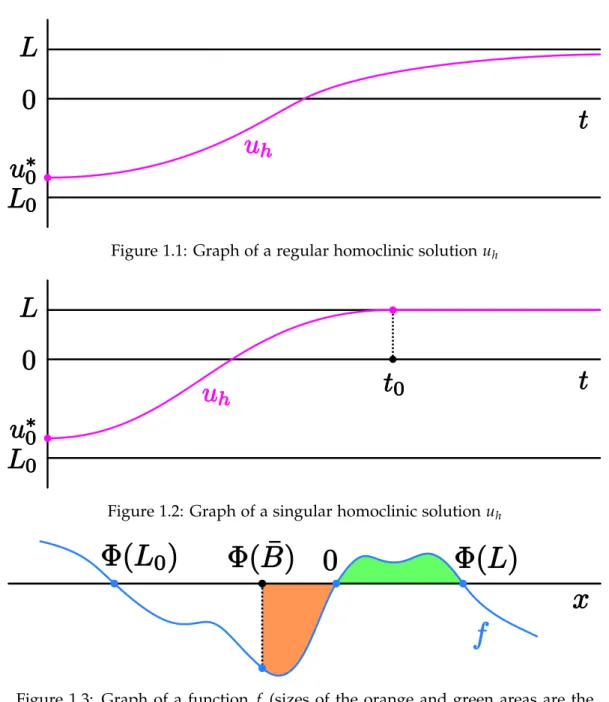
If usup = L and u is nondecreasing (i.e. limt→_∞u(t) = L), then u is called a homoclinic solutionof IVP (1.1), (1.2).

The homoclinic solution is called aregular homoclinic solution, ifu(t)< Lfort∈ [0,∞)and asingular homoclinic solution, if there existst₀ >0 such thatu(t) =Lfort∈ [t₀,∞).

Ifu_sup > L, thenuis called anescape solutionof IVP (1.1), (1.2).

Conditions giving the existence of damped solutions are published in [5] nad those for the existence of escape solutions can be found in [25]. Our goal is to prove the existence of a homoclinic solution of IVP (1.1), (1.2) with some starting valueu₀ ∈ [L₀, 0) provided some suitable additional conditions are fulfilled. The main result of the paper is contained in the next theorem.

Theorem 1.5(Homoclinic solutions). Let(1.3)–(1.7)and(2.2)–(2.4)hold. Further assume that there exists a right neighbourhood ofφ(L₀), where f is decreasing. (1.11) Then there exists u^∗₀ ∈[L₀, ¯B)such that a solution u_h of IVP(1.1),(1.2)with u₀= u^∗₀ is homoclinic.

Examples of graphs of homoclinic solutions and of a function f satisfying the conditions of Theorem1.5are in Figures1.1–1.3.

2 Auxiliary results

Here we present an overview of results from [5] and [25] which we need to get a homoclinic solution of IVP (1.1), (1.2). The first group consists of results about existence and uniqueness which follow from [5, Th. 4.1, Th. 5.1, Th. 5.4, Th. 6.5] and [25, Th. 4.7].

Since values of any homoclinic solution belong to[L₀,L], we can assume without loss of generality

f(x) =0 for x≤φ(L₀), x≥φ(L) (2.1) in our next investigation.

Figure 1.1: Graph of a regular homoclinic solutionu_h

Figure 1.2: Graph of a singular homoclinic solutionu_h

Figure 1.3: Graph of a function f (sizes of the orange and green areas are the same)

Theorem 2.1(Existence of solutions). Assume(1.3)–(1.7) and(2.1). Then, for each starting value u₀ ∈[L₀, 0), there exists a solution of IVP(1.1),(1.2).

Theorem 2.2(Damped solutions). Let(1.3)–(1.7)and(2.1)hold and let

∃B^¯ ∈ (L₀, 0): F(B^¯) =F(L), where F(x) =

Z _x

0 f(φ(s))ds, x∈_R, (2.2) and

tlim→_∞

p⁰(t)

p(t) =0. (2.3)

Then every solution of IVP(1.1),(1.2)with the starting value u₀∈ [B, 0^¯ )is damped.

Assume in addition that

limx→0|x|φ⁻¹ 0

(x)<_∞, (2.4)

and that u is a damped solution of IVP (1.1), (1.2)with the starting value u₀ ∈ (L₀, 0). Then u is a unique solution of this IVP.

Theorem 2.3 (Escape solutions). Let (1.3)–(1.7) and (2.1)–(2.3) hold. Then there exist infinitely many escape solutions of IVP(1.1),(1.2)with starting values in[L0, ¯B).

Assume in addition that (2.4) hold and that u is an escape solutions of IVP(1.1), (1.2) with the starting value u₀ ∈(L₀, ¯B). Then u is a unique solution of this IVP.

Remark 2.4. The uniqueness of damped and escape solutions is proved in [5, Th. 5.4, Th. 6.5]

under the assumptions (1.9), (1.10). Using the arguments from the proof of Lemma4.1, we see that the requirement of the monotonicity ofφ⁰ can be omitted and (1.9), (1.10) can be replaced with (2.4).

Remark 2.5. If we assume that (1.3)–(1.7) and (2.1)–(2.3) hold and in addition that φ⁰(0)>0, then the condition

φ⁻¹∈Lip_loc(_R), (2.5)

is fulfilled. In this case, by Theorem 2.1 and [5, Th. 4.3], for each u₀ ∈ [L₀, 0) there exists a unique solution of IVP (1.1), (1.2). In particular for u₀ = L₀ IVP (1.1), (1.2) has a unique (constant) solution.

Example 2.6. As an example ofφsatisfying (1.3), (1.4) andφ⁰(₀)>0 we choose φ(x) =sinh(x) = (e^x−e^−x)/2, x∈_R.

The second group contains results about asymptotic behaviour of damped, escape and ho- moclinic solutions and can be reached from [5, L. 2.1b), L. 2.6, L. 2.8, L. 3.2, L. 3.4, L. 6.2, L. 6.3]

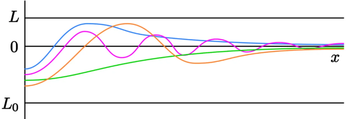
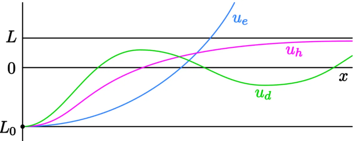
and [25, L. 3.3, L. 3.4]. In particular, paper [5] mostly deals with damped solutions and proves their possible behaviour as illustrated in Figure 2.1. Paper [25] investigates escape solutions, proves their monotonicity and presents conditions guaranteeing their unboundedness. For graphs of escape solutions see Figure2.2.

Figure 2.1: Graphs of damped solutions

Theorem 2.7(Starting value in (L0, 0)). Let(1.3)–(1.7) and(2.1)–(2.3) hold and let u be a solution of IVP(1.1),(1.2)with the starting value u₀ ∈(L₀, 0). Then

u(t)> L₀ and ∃c˜>0 such that|u⁰(t)| ≤c˜ for t ∈(0,∞). (2.6) The constantc depends on L˜ ₀, L₁,φand f and does not depend on p and u.

Figure 2.2: Graphs of escape solutions 1. Assume that u_sup < L, i.e. u is a damped solution.

• Letθ >0be the first zero of u. Then there existsθ < a<b such that

u(a)∈(0,L), u⁰(t)>0 on(0,a), u⁰(a) =0, u⁰(t)<0 on(a,b). (2.7)

• Let u<0on[0,∞). Then

u⁰(t)>0 for t ∈(0,∞), lim

t→_∞u(t) =0, lim

t→_∞u⁰(t) =0. (2.8) 2. Assume that usup > L, i.e. u is an escape solution. Then

u⁰(t)>0 for t∈(0,∞). (2.9) 3. Assume that usup = L. Then there are two possibilities.

• u(t)<L for t ∈[0,∞)which yields

u⁰(t)>0 for t ∈(0,∞), lim

t→_∞u(t) = L, lim

t→_∞u⁰(t) =0, (2.10) and u is a regular homoclinic solution.

• There exists t₀>0such that u(t₀) =L, u⁰(t₀) =0which implies

u⁰(t)>0 for t ∈(0,t0), (2.11) and there exists a singular homoclinic solution v, where v = u on [0,t₀] and v = L on [t0,∞).

Consider a solutionu 6≡L₀of IVP (1.1), (1.2) withu₀= L₀. SinceL₀<0, there existsε>0 such thatu(t)<0 fort∈[0,ε], and by (2.1), f(φ(u(t)))≤0 fort ∈[0,ε]. Integrating (1.1) over [0,t]we get

p(t)φ(u⁰(t)) =−

Z _t

0 p(s)f(φ(u(s)))ds≥0, t ∈[0,ε].

Henceu⁰(t)≥0 andu(t)is nondecreasing on [0,ε]. Consequently, sinceu6≡L₀, there exists a maximala0≥0 such that

u(t) =L₀ on [0,a₀]anduis increasing in a right neighbouhood of a₀. (2.12) The next theorem describes asymptotic behaviour of damped, homoclinic and escape solutions starting atL₀, which is the same as that of solutions with starting values greater than L₀.

Theorem 2.8(Starting value L₀). Let(1.3)–(1.7)and(2.1)–(2.3)hold and let u be a solution of IVP (1.1),(1.2)with the starting value u0 =L0. Further, let u 6≡L0and let a0 ≥0be from(2.12). Then

u(t)>L₀ and ∃c˜>0 such that|u⁰(t)| ≤c˜ for t∈ (a₀,∞). (2.13) The constantc depends on L˜ ₀, L₁,φand f and does not depend on p and u.

1. Assume that usup < L, i.e. u is a damped solution.

• Letθ >a₀be the first zero of u. Then there existθ <a <b such that

u(_a) = (_0,L)_{, u}⁰(_t)>_{0 on}(_a0,a)_{, u}⁰(_a) =_{0, u}⁰(_t)<_{0 on} (_a,b)_{. (2.14)}

• Let u<₀on[_0,∞). Then

u⁰(t)>0 on(a₀,∞), lim

t→_∞u(t) =0, lim

t→_∞u⁰(t) =0. (2.15) 2. Assume that u_sup > L, i.e. u is an escape solution. Then

u⁰(t)>0 for t∈(a₀,∞). (2.16) 3. Assume that usup = L. Then there are two possibilities.

• u(t)< L for t∈ [0,∞)which yields

u⁰(t)>0 for t∈ (a0,∞), lim

t→_∞u(t) =L, lim

t→_∞u⁰(t) =0, (2.17) and u is a regular homoclinic solution.

• There exists t₀ >a₀such that u(t₀) =L, u⁰(t₀) =0which implies

u⁰(t)>0 for t∈(a₀,t₀), (2.18) and there exists a singular homoclinic solution v, where v = u on[0,t₀] and v = L on [t₀,∞).

3 Escape solution and damped solution start in ( L

, 0 )

In this section we derive further needed properties of escape and homoclinic solutions.

Assume (1.3)–(1.7), (2.1)–(2.4) hold and define sets

M_e= {u₀∈ (L₀, 0)_:u is an escape solution of IVP (1.1), (1.2)}_{, (3.1)} M_d ={u₀ ∈(L₀, 0):uis a damped solution of IVP (1.1), (1.2)}. (3.2) By Theorem 2.2, the set M_d is nonempty. In this section we assume that the set M_e is also nonempty and prove that the sets M_e and M_d are open in (L₀, 0). These properties ofM_e andM_dare used in Section5in the proof of Theorem1.5.

Lemma 3.1. Let(1.3)–(1.7) and(2.1)–(2.4) hold. Assume that B ∈ [L₀, 0),B_n ∈ (L₀, 0)for n ∈ _N and

nlim→_∞Bn=B.

Further, let u_nbe a solution of IVP(1.1),(1.2)with u₀ = B_n, n ∈N, and let u be a damped solution or an escape solution of IVP(1.1),(1.2)with u₀ =B. Then for each b>0

nlim→_∞u_n(t) =u(t) uniformly on [0,b]. (3.3)

Proof. Since eachu_nfulfils (1.1) we get after integration u_n(t) =B_n+

Z _t

0

φ⁻¹

− ¹ p(s)

Z _s

0

p(τ)f(φ(u_n(τ)))_dτ

ds, t ∈[_0,∞)_, n∈_{N. (3.4)} Choose an arbitraryb>0. By (2.6) the sequence{u_n}is bounded and equicontinuous on[0,b] and by the Arzelà–Ascoli Theorem there exists a subsequence{u_k} ⊂ {u_n}which uniformly converges on[0,b]to a continuous functionv. Hence the limitvfulfils

v(t) =B+

Z _t

0 φ⁻¹

− ¹ p(s)

Z _s

0 p(τ)f(φ(v(τ)))dτ

ds, t∈[0,b].

So,vis a solution of IVP (1.1), (1.2) withu₀= B. By Theorems2.2or2.3, we getu=von[0,b] and (3.3) follows.

Lemma 3.2. Let(1.3)–(1.7)and(2.1)–(2.4)hold. Then the setM_efrom(3.1)is open in(L₀, 0). Proof. Let us choose an arbitrary B ∈ M_e. Then the corresponding solution u of IVP (1.1), (1.2) withu0 =_Bis an escape solution and so there exists b>0 such thatu(_b)> _L.

Assume that in any neighbourhood of B there exist starting values of solutions which are not escape solutions. Then we get a sequence {B_n} ⊂ (L₀, 0) converging to B and a corresponding sequence{un}of solutions of IVP (1.1), (1.2) withu0 = Bn satisfying (3.3). In additionu_n≤ Lon [0,∞)forn∈ N. By (3.3) we getu(b)≤ L, a contradiction. Therefore for eachB∈ M_ethere exists a neighbourhood ofBbelonging toM_e.

Lemma 3.3. Let(1.3)–(1.7)and(2.1)–(2.4)hold. Then the setM_dfrom(3.2)is open in(L₀, 0). Proof. Let us choose an arbitrary B ∈ M_d. Then the corresponding solution u of IVP (1.1), (1.2) withu₀ =Bis a damped solution.

Assume that in any neighbourhood ofBthere exist starting values of solutions which are not damped solutions. By Theorem2.7we get a sequence {Bn} ⊂(L₀, 0)converging toBand a corresponding sequence {u_n} of nondecreasing solutions of IVP (1.1), (1.2) with u₀ = B_n satisfying (3.3). Thereforeuis also nondecreasing.

1. Assume thatu has a zero θ > 0. By (2.7) there existθ < a < b such that u(a) ∈ (0,L) anduis decreasing on[a,b], a contradiction.

2. Assume thatu<_{0 on}[_0,∞). Then (1.1) yields φ⁰(u⁰(t))u⁰(t)u⁰⁰(t) + ^p

0(t)

p(t)^φ(u⁰(t))u⁰(t) + f(φ(u(t)))u⁰(t) =0, t>0. (3.5) Integrating (3.5) from 0 tot >0 and using (2.2) and (2.8) we get

Z _u⁰_(t)

0 xφ⁰(x)dx+

Z _t

0

p⁰(s)

p(s)^φ(u⁰(s))u⁰(s)ds= F(B)−F(u(t)), t >0, (3.6) and fort→_∞

Z _∞

0

p⁰(s)

p(s)^φ(u⁰(s))u⁰(s)ds= F(B)∈(0,∞). (3.7) Consequently there existb>_{0 and}η>0 such that

Z _∞

b

p⁰(s)

p(s)^φ(u⁰(s))u⁰(s)ds<η< ^F(L)

3 . (3.8)

Hence (3.7) and (3.8) give Z _b

0

p⁰(s)

p(s)^φ(u⁰(s))u⁰(s)ds> F(B)−η. (3.9) (i) Assume for each n ∈ N, that starting value Bn can be chosen such that the corre- sponding solution u_n is not a singular homoclinic solution. So,u_nis either escape or regular homoclinic solution, and forn∈ _N, we get similarly as in (3.6)

Z _u⁰_n(t)

0 xφ⁰(x)dx+

Z _t

0

p⁰(s)

p(s)^φ(u⁰_n(s))u⁰_n(s)ds= F(B_n)−F(u_n(t)), t >0, (3.10) and so

F(u_n(t))< F(B_n)−

Z _b

0

p⁰(s)

p(s)^φ(u⁰_n(s))u⁰_n(s)ds, t >b. (3.11) Using (3.9) we derive an estimation for the integral in (3.11) as follows. We have

Z _b

0

p⁰(s)

p(s)^φ(u⁰_n(s))u⁰_n(s)ds>

Z _b

0

p⁰(s)

p(s) ^φ(u⁰_n(s))u⁰_n(s)−φ(u⁰(s))u⁰(s) ds+F(B)−η, and due to (3.6) and (3.10),

Z _b

0

p⁰(s)

p(s) ^φ(u⁰_n(s))u⁰_n(s)−φ(u⁰(s))u⁰(s) ds

= F(B_n)−F(B) +F(u(b))−F(u_n(b)) +

Z _u⁰_(b)

u⁰_n(b) xφ⁰(x)dx.

Therefore, (3.11) yields

F(un(t))<|F(u(b)−F(un(b))|+

Z _u⁰_(b)

u⁰_n(b) xφ⁰(x)dx

+η, t>b.

By (3.3) and (3.4),

nlim→_∞F(un(b)) =F(u(b)), lim

n→_∞u⁰_n(b) =u⁰(b), and so if nis sufficiently large, then

F(u_n(t))<3η< F(L), t >b.

By (2.2) the function F(x) is increasing for x ∈ (0,∞), and so if 0 < un(t) then un(t) <

F⁻¹(3η)< Lfort >b. Consequently, sinceu_nis increasing on[0,∞)we haveu_n< F⁻¹(3η)<

Lon[0,∞)which contradicts the assumption thatu_n is an escape or regular homoclinic solu- tion.

(ii) Let B_n, n ∈ N, be such that the corresponding solutions u_n, n ∈ N, are singular homoclinic solutions. According to Theorem 2.7 there exists a sequence {t_n} ⊂ (_0,∞) _such that

u⁰_n(t)>0, t ∈(0,t_n), u⁰_n(t_n) =0, u_n(t) =L, t∈[t_n,∞), n∈_N. (3.12) Let there exist c ∈ (0,∞) such that t_n ≤ c, and hence u_n(c) = L, n ∈ N. Then (3.3) yields u(c) = L. Since we assumed that u < _{0 on} [_0,∞), we get a contradiction. Therefore there exists a subsequence {t_k} ⊂ {tn}going to ∞, and for b from (3.8) we get t_k > b fork ≥ k₀, with a sufficiently large k₀. Similarly as in (3.10) and (3.11) we derive

Z _u⁰

k(t)

0 xφ⁰(x)dx+

Z _t

0

p⁰(s)

p(s)^φ(u⁰_k(s))u⁰_k(s))ds =F(B_k)−F(u_k(t)), t ∈(0,t_k), k≥k₀,

F(u_k(t))<F(B_k)−

Z _b

0

p⁰(s)

p(_s)^φ(u⁰_k(s))u⁰_k(s)ds, t ∈(b,t_k), k≥k₀. (3.13) We derive the estimation of the integral in (3.13) as in (i) and get for a sufficiently large kthe estimateu_k(t_k)≤ F⁻¹(3η)< Lcontrary to (3.12).

We have proved that for each B ∈ M_d there exists a neighbourhood of B belonging to M_d.

4 Escape solution and damped solution start at L

If we have not an escape solution of IVP (1.1), (1.2) starting at u₀ > L₀, we need some further properties of escape and damped solutions starting atL₀.

Assume (1.3)–(1.7), (1.11) and (2.1)–(2.4) hold and denote by S the set of all damped, escape and homoclinic solutions of IVP (1.1), (1.2) with the starting valueu0 = _{L0. Let ue be} an escape solution and u_d 6≡ L₀ be a damped solution of IVP (1.1), (1.2). In this section we assume that

ue,u_d∈ S. (4.1)

According to (1.11) there exists C ∈ (L₀, 0) such that f is decreasing on [φ(L₀),φ(C)]. By Theorem 2.8 there exist minimal γ_d > 0 and minimal γ_e > 0 such that u_d(γ_d) = C and ue(γe) =C. Let us put

γ₀=min{γ_e,γ_d}. (4.2)

Lemma 4.1. Let(1.3)–(1.7),(1.11) and(2.1)–(2.4)hold. Then for each γ ≥ γ₀ there exists a unique solution u_γ ∈ S satisfying u_γ(γ) =C. Further there exists a_γ ∈[0,γ)such that

uγ(t) =L₀ on[0,aγ], uγ(t)∈(L₀,C) on(aγ,γ). (4.3) Proof. The existence follows from Lemma 4.6 in [25] where it is proved by the lower and upper functions method. Theorem2.8yields (4.3). It remains to prove the uniqueness.

Step 1.Let us show that

γ₀ ≤γ₁< γ₂ =⇒ a_γ1 ≤ a_γ2. (4.4) Assume on the contrary thata_γ1 > a_γ2, so the graphs ofu_γ1 andu_γ2 intersect and there exists ξ ∈(aγ₁,γ₁)such that

u_γ1(t) =u_γ2(t) = L₀ on [_0,a_γ2]_, u_γ1(t)<u_γ2(t) _on(a_γ2,ξ)_, u_γ1(ξ) =u_γ2(ξ)∈ (L₀,C)_. Consequently,

u⁰_γ1(ξ)≥u⁰_γ2(ξ). (4.5) On the other hand, since f is decreasing on[φ(L₀),φ(C)]we get due to (1.3)−f(φ(uγ₂(t)))>

−f(φ(u_γ1(t)))fort∈ (a_γ2,ξ). Sinceu_γi satisfy (1.1), we get by integration over[0,ξ] φ u⁰_γi(ξ)=− ¹

p(ξ)

Z _ξ

0

p(s)f(φ(u_γi(s)))ds, i=_{1, 2,} soφ u⁰_γ2(ξ)>φ u⁰_γ1(ξ) andu⁰_γ2(ξ)> u⁰_γ1(ξ), contrary to (4.5).

Step 2. Now, assume that for some γ ≥ γ₀ there exist two different solution u₁,u₂ ∈ S such that u₁(γ) = u₂(γ) = C. Similarly as in Step 1 we get that the graphs of u₁ and u₂ cannot intersect. Therefore there exists an interval(τ₀,τ₁)⊂ (_0,γ)_{such that} u₁ > u₂ on (τ₀,τ₁)_and

u₁(τ₀) = u₂(τ₀), u⁰₁(τ₀) = u⁰₂(τ₀), u₁(τ₁) = u₂(τ₁). Then u⁰₁(τ₁) ≤ u⁰₂(τ₁). Since u₁,u₂ are solutions of (1.1), it holds

(p(t)φ(u⁰_i(t)))⁰+p(t)f(φ(u_i(t))) =0, t∈ (0,∞), i=1, 2. (4.6) Integrating (4.6) over[τ₀,τ₁]we have

p(τ₁)φ u⁰_i(τ₁)= p(τ₀)φ u⁰_i(τ₀)−

Z _τ1

τ₀

p(s)f(φ(u_i(s)))ds, i=1, 2, which impliesu₂⁰(τ₁)<u⁰₁(τ₁), a contradiction. We have proved that

u₁(t) =u₂(t) fort∈ [0,γ]. (4.7) Step 3. Integrating (4.6) over[γ,t]we get fort >γ

φ(u⁰_i(t)) = ^p(γ)

p(t)^φ(u⁰_i(γ))− ¹ p(t)

Z _t

γ

p(s)f(φ(u_i(s)))ds=: A_i(t), i=1, 2, and so

u⁰_i(t) =φ⁻¹(A_i(t)), u_i(t) =C+

Z _t

γ

φ⁻¹(A_i(s))ds, i=1, 2.

By Theorem2.8there exist β> γandc₀, ˜csuch that

0<c₀≤ u⁰_i(t)≤c,˜ u_i(t)∈ (L₀,L), t∈[γ,β], i=1, 2. (4.8) Then 0 < φ(c0) < A_i(t) ≤ φ(c˜) fort ∈ [γ,β], i = 1, 2. Therefore, due to (1.3), there exists a Lipschitz constant Λ_φ⁻¹ of the functionφ⁻¹ on the interval[φ(c₀),φ(c˜)]such that

|u⁰₁(t)−u⁰₂(t)| ≤_Λφ−1|A₁(t)−A₂(t)|_, |u₁(t)−u₂(t)| ≤_Λφ−1

Z _t

γ

|A₁(s)−A₂(s)|ds, t∈[_γ,β]_. In addition, by (1.3) and (1.6) we can find Lipschitz constants Λφ and Λf of the functions φ and f on the intervals[L₀,L]and[φ(L₀),φ(L)], respectively. Hence, by (1.7), (4.7) and (4.8),

|A₁(t)−A2(t)| ≤ ¹ p(t)

Z _t

γ

p(s)|f(φ(u2(s)))− f(φ(u₁(s)))|ds

≤_ΛfΛφ

Z _t

γ

|u₂(s)−u₁(s)|ds, t ∈[γ,β]. This implies

|u₁(t)−u2(t)| ≤_Λφ−1ΛfΛφ(β−γ)

Z _t

γ

|u₁(s)−u2(s)|ds, t∈ [γ,β], and the Gronwall lemma yields

u₁(t) =u₂(t) fort ∈[γ,β]. (4.9) Let β^∗ be a supremum of all suchβsatisfying (4.8). Let us denoteρ(t)_:=u₁(t)−u₂(t)_{. Then} by (4.7) and (4.9)

ρ(t) =0 fort∈ [0,β^∗). (4.10) If β^∗ =_{∞, then}u₁ =u₂ on[_0,∞)and the uniqueness is proved.

Step 4. Let β^∗ < _{∞. Since}ρ ∈C¹[0,∞), it holdsρ(β^∗) =0,ρ⁰(β^∗) =0 due to (4.10), and u₁,u₂ reachLatβ^∗ or u⁰₁,u⁰₂ reach 0 atβ^∗.

(i) Letu₁(β^∗) =u₂(β^∗) =Landu⁰₁(β^∗) =u⁰₂(β^∗)>0. Thenu₁andu₂are escape solutions, and by (2.1), we obtain by integration of (4.6) over[β^∗,t]

φ(u⁰₁(t)) = ^p(β^∗)

p(t) ^φ(u⁰₁(β^∗)) =φ(u⁰₂(t)), t≥ β^∗. Thereforeu⁰₁ =u⁰₂ on[β^∗,∞)and

u₁(t) =L+

Z _t

β^∗

φ⁻¹

p(β^∗)

p(s) ^φ(u⁰₁(β^∗))

ds= u₂(t), t ≥β^∗. (4.11) (ii) Let u₁(β^∗) = u₂(β^∗) = L and u⁰₁(β^∗) = u⁰₂(β^∗) = 0. Then u₁ and u₂ are singular homoclinic solutions, and

u₁(t) =L=u₂(t)_, t≥ β^∗. (4.12) To summarize, in the both cases (i) and (ii) the uniqueness is proved.

(iii) Let u₁(β^∗) = u₂(β^∗) < L and u⁰₁(β^∗) = u⁰₂(β^∗) = 0. Then u₁ and u₂ are damped solutions and by Theorem2.8 there existsb > β^∗ such that u₁,u₂ are decreasing and positive on[β^∗,b]. Therefore

min{f(φ(u_i(t))):t ∈[β^∗,b]}=:K_min >0, max{f(φ(u_i(t))):t ∈[β^∗,b]}=:K_max <_∞.

Integrating (4.6) over[β^∗,t], we get fort >β^∗ φ u⁰_i(t) =− ¹

p(t)

Z _t

β^∗

p(s)f(φ(u_i(s)))ds=:A_i^∗(t), i=1, 2, and hence

−Kmax

Z _t

β^∗

p(s)

p(t)^ds ≤ A^∗_i(t)≤ −Kmin

Z _t

β^∗

p(s)

p(t)^{ds, t}∈ (β^∗,b]. (4.13) Consequently, there exists a functionKwith

K_min ≤K(t)≤K_max fort∈ (β^∗,b]_, such that

|φ⁻¹(A^∗₁(t))−φ⁻¹(A^∗₂(t))| ≤φ⁻¹ 0

−K(t)

Z _t

β^∗

p(s) p(_t)^ds

|A^∗₁(t)−A^∗₂(t)|, t ∈(β^∗,b]. Due to (2.4), there existsK_φ >0 such that

0<|x|φ⁻¹ 0

(x)≤ Kφ, x∈[−1, 0), (4.14) and sinceK is bounded, there existsδ∈ (β^∗,b)such that

−₁≤ −K(t)

Z _t

β^∗

p(s)

p(t)^ds<_0, t ∈(β^∗,δ]_. Clearly, forx =−K(t)Rt

β^∗ p(s)

p(t)dsin (4.14), we obtain 0<_K(_t)

Z _t

β^∗

p(s) p(t)^ds

φ⁻¹

0

−K(_t)

Z _t

β^∗

p(s) p(t)^ds

≤Kφ, t ∈(β^∗,δ]_{. (4.15)}

Denote

ρ(t):=max{|u₁(s)−u₂(s)|:s∈[β^∗,t]}, t∈[β^∗,δ]}. Since

u_i(t) =u_i(β^∗) +

Z _t

β^∗

φ⁻¹(A_i^∗(s))ds, i=1, 2, and

|A^∗₁(t)−A^∗₂(t)| ≤ ¹ p(t)

Z _t

β^∗

p(s)|f(φ(u₂(s))− f(φ(u₁))|ds ≤ρ(t)_ΛfΛφ

Z _t

β^∗

p(s) p(t)^ds, we get by (4.15)

ρ(t)≤ ^Kφ

K_minΛfΛφ

Z _t

β^∗

ρ(s)ds, t ∈[β^∗,δ]. The Gronwall lemma yields

u₁(t) =u₂(t) _fort∈[β^∗,δ]_{. (4.16)} Modifying and repeating the arguments from Steps 3–5 we get the uniqueness in case (iii).

Define sets

Γe ={γ∈[γ₀,∞):u_γ ∈ S is an escape solution andu_γ(γ) =C}, (4.17) Γd={γ∈ [γ₀,∞):uγ ∈ S is a damped solution anduγ(γ) =C}. (4.18) According to (4.1) the setsΓe,Γd are nonempty. We prove that these sets are open in[γ₀,∞), which we need in the proof in Section 5.

Lemma 4.2. Let (1.3)–(1.7), (1.11) and (2.1)–(2.4) hold. For n ∈ _N consider γ_n ∈ (γ₀,∞) and u_γn ∈ Swith u_γn(γ_n) =C. Assume that

nlim→_∞γn= γ∈[γ₀,∞). Then for each b>γ

nlim→_∞u_γn(t) =u_γ(t) uniformly on[0,b], u_γ ∈ S and u_γ(γ) =C. (4.19) Proof. Since eachuγn fulfils (1.1) we get after integration

u_γn(t) =L₀+

Z _t

0 φ⁻¹

− ¹ p(s)

Z _s

0 p(τ)f(φ(u_γn(τ)))dτ

ds, t ∈[0,∞), n∈_N. (4.20) Choose an arbitrary b > γ. By (2.13) the sequence {u_γn} is bounded and equicontinuous on [_0,b]and by the Arzelà-Ascoli Theorem there exists a subsequence {u_γk} ⊂ {u_γn}_which uniformly converges on [0,b] to a continuous function v. Hence the limit v fulfils v(γ) = C and

v(t) = L₀+

Z _t

0 φ⁻¹

− ¹ p(s)

Z _s

0 p(τ)f(φ(v(τ)))dτ

ds, t ∈[0,b]. So,v∈ S_{. By Lemma4.1we get}v=u_γ on[_0,b], and (4.19) follows.

Remark 4.3. Consider u_γ and the sequence {u_γn} from Lemma 4.2. Since u_γ(γ) = C and uγn(γ_n) = C, we have uγ 6≡L0 anduγn 6≡ L0,n ∈ N. So, according to (2.12) and (4.19), there exist maximala₀∈[0,γ)anda_n∈ [0,γ_n)such that

u_γ(t) =L₀ fort∈[0,a₀], u_γn(t) = L₀ fort∈ [0,a_n], n∈_N, lim

n→_∞a_n=a₀. (4.21) Lemma 4.4. Let(1.3)–(1.7),(1.11)and(2.1)–(2.4)hold. Then the setΓefrom(4.17)is open in[γ₀,∞). Proof. Let us choose an arbitrary γ ∈ _Γe. Then the corresponding solution u_γ ∈ S with uγ(γ) =Cis an escape solution and so there existsb>γsuch thatuγ(b)> L.

Assume that there exist a sequence {γn} ⊂(γ₀,∞)converging to γ and a corresponding sequence of non-escape solutions{u_γn} ⊂ S with u_γn(γ_n) = C. By Lemma 4.2, the sequence {u_γn} uniformly converges tou_γ on [_0,b]_{. Since}u_γn(b) ≤ L, we get u_γ ≤ L, a contradiction.

Therefore for eachγ∈_Γethere exists a neighbourhood ofγin[γ₀,∞)belonging toΓe.

Lemma 4.5. Let(1.3)–(1.7),(1.11)and(2.1)–(2.4)hold. Then the setΓdfrom(4.18)is open in[γ₀,∞). Proof. Let us choose an arbitrary γ ∈ _Γd. Then the corresponding solution uγ ∈ S with u_γ(γ) =Cis a damped solution.

Assume that there exist a sequence {γ_n} ⊂(γ₀,∞)converging to γ and a corresponding sequence of non-damped solutions {uγn} ⊂ S with uγn(γ_n) = C. Due to Remark 4.3, the conditions (4.21) hold. By Theorem 2.8, eachuγn is nondecreasing on [0,∞). By Lemma4.2 the sequence{u_γn}uniformly converges tou_γ on[0,b]for anyb>γ. Thereforeu_γ is nonde- creasing on[0,∞).

1. Assume thatuγhas a zeroθ > a₀. By (2.14) there existθ< a<bsuch thatuγ(a)∈(0,L) andu_γ is decreasing on[a,b], a contradiction.

2. Assume thatu_γ<0 on [0,∞). Then (1.1) yields φ⁰(u⁰_γ(t))u⁰_γ(t)u⁰⁰_γ(t) + ^p

0(t)

p(t)^φ(u⁰_γ(t))u⁰_γ(t) + f(φ(uγ(t)))u⁰_γ(t) =0, t>a₀. (4.22) Integrating (4.22) froma₀tot> a₀, using (2.2), (2.15) and arguing as in the proof of Lemma3.3, we get

Z _u⁰_γ(t)

0 xφ⁰(x)dx+

Z _t

a0

p⁰(s)

p(s)^φ(u⁰_γ(s))u⁰_γ(s)ds =F(L₀)−F(uγ(t)), t> a₀, (4.23) and fort→_∞

Z _∞

a₀

p⁰(s)

p(s)^φ(u⁰_γ(s))u⁰_γ(s)ds= F(L₀)∈(0,∞). (4.24) Consequently there existb> a₀,b>a_n,n∈_{N, and}η>0 such that

Z _∞

b

p⁰(s)

p(s)^φ(u⁰_γ(s))u⁰_γ(s)ds <η< ^F(L)

3 . (4.25)

Hence (4.24) and (4.25) give Z _b

a0

p⁰(s)

p(s)^φ(u⁰_γ(s))u⁰_γ(s)ds> F(L₀)−η. (4.26)

(i) Assume for eachn∈_{N, that}γ_n∈ (γ₀,∞)can be chosen such that the corresponding so- lutionuγn is not a singular homoclinic solution. So,uγn is either escape or regular homoclinic solution, and forn ∈N, we get similarly as in (4.23)

Z _u⁰

γn(t)

0 xφ⁰(x)dx+

Z _t

an

p⁰(s)

p(s)^φ(u⁰_γn(s))u⁰_γn(s)ds= F(L₀)−F(u_γn(t)), t >a_n, (4.27) and so

F(uγn(t))< F(L0)−

Z _b

an

p⁰(s)

p(s)^φ(u⁰_γn(s))u⁰_γn(s)ds, t >b. (4.28) Using (4.26) we derive an estimation for the integral in (4.28) as follows. We have

Z _b

an

p⁰(s)

p(s)^φ(u⁰_γn(s))u⁰_γn(s)ds

>

Z _b

an

p⁰(s)

p(s)^φ(u⁰_γn(s))u⁰_γn(s)ds−

Z _b

a₀

p⁰(s)

p(s)^φ(u⁰_γ(s))u⁰_γ(s)ds+F(L₀)−η, and due to (4.23) and (4.27),

Z _b

an

p⁰(s)

p(s)^φ(u⁰_γn(s))u⁰_γn(s)ds−

Z _b

a0

p⁰(s)

p(s)^φ(u⁰_γ(s))u⁰_γ(s)ds

= F(uγ(b))−F(uγn(b)) +

Z _u⁰

γ(b)

u⁰_γn(b)xφ⁰(x)dx.

Therefore, (4.28) yields

F(u_γn(t))<|F(u_γ(b)−F(u_γn(b))|+

Z _u⁰

γ(b)

u⁰_γn(b)xφ⁰(x)dx

+η, t>b.

By (4.19) and (4.20),

nlim→_∞F(uγn(b)) =F(uγ(b)), lim

n→_∞u⁰_γn(b) =u⁰_γ(b), and so if nis sufficiently large, then

F(uγn(t))<3η<F(L), t>b.

We get a contradiction as in part (i) of the proof of Theorem3.3.

(ii) Let γ_n, n ∈ N, be such that the corresponding solutions uγn, n ∈ N, are singular homoclinic solutions. According to Theorem 2.8, forn ∈ N, there exists a t_n ∈ (a_n,∞)such that

u⁰_γn(t)>0, t ∈(a_n,t_n), u⁰_γn(t_n) =0, uγn(t) =L, t∈ [t_n,∞), n∈_N.

Then we argue similarly as in part (ii) of the proof of Theorem3.3(working on(a_k,t_k)instead of (0,t_k)) and derive a contradiction.

We have proved that for eachγ∈_Γdthere exists a neighbourhood ofγin[γ₀,∞)belonging to Γd.