About existence and regularity of positive solutions for a quasilinear Schrödinger equation

About existence and regularity of positive solutions for a quasilinear Schrödinger equation

with singular nonlinearity

Ricardo Lima Alves

and Mariana Reis

1Departamento de Matemática, Universidade de Brasília-UnB, CEP: 70910-900, Brasília-DF, Brazil

2Departamento de Matemática, Universidade Federal da Integração Latino-Americana, Av. Tancredo Neves, 6731, PO Box 2044 - CEP 85.867-970, Foz do Iguaçu-Paraná, Brazil

Received 19 May 2020, appeared 28 October 2020 Communicated by Gabriele Bonanno

Abstract. We establish the existence of positive solutions for the singular quasilinear Schrödinger equation

(−∆u−∆(u²)u=h(x)u^−γ+f(x,u) inΩ,

u(x) =0 on∂Ω,

where Ω ⊂ R^N (N ≥ 3) is a bounded domain with smooth boundary ∂Ω, 1 < _γ, h ∈ L¹(_Ω) and h > 0 almost everywhere in Ω. The function f may change sign on Ω. By using the variational method and some analysis techniques, the necessary and sufficient condition for the existence of a solution is obtained.

Keywords: strong singularity, variational methods, regularity, fibering methods, indef- inite nonlinearity.

2020 Mathematics Subject Classification: 35J62, 35J20, 55J75.

1 Introduction

In this paper we study the existence of solution for the following quasilinear Schrödinger equation











−_∆u−_∆(u²)u=h(x)u^−γ+ f(x,u) inΩ,

u>0 inΩ,

u(x) =0 on∂Ω,

(P)

where Ω⊂ _R^N(N ≥ 3)is a bounded domain with smooth boundary∂Ω, 1< γ, h ∈ L¹(_Ω), h > 0 almost everywhere (a.e.) in Ω and f : Ω×_R −→ _R is a Carathéodory function. We assume that the function f satisfies one of the following conditions:

(f)₁ f(x,s) =b(x)s^p, where p ∈(_{0, 1})_,b∈ L^∞(_Ω)_andb⁺=_max{b, 0} 6≡0.

BCorresponding author. Email: ricardoalveslima8@gmail.com

(f)₂ f(x,s) =−b(x)s^22∗−1, whereb∈L^∞(_Ω)andb≥0 a.e. inΩ.

We say that a function u ∈ H₀¹(_Ω) is a weak solution (solution, for short) of (P) if u > 0 a.e. inΩ, and, for everyϕ∈ H₀¹(_Ω),

hu^−γϕ∈ L¹(_Ω) (1.1)

and _Z

Ω[(1+2u²)∇u∇ϕ+2u|∇u|²ϕ] =

Z

Ωh(x)u^−γϕ+

Z

Ω f(x,u)ϕ.

Consider the following quasilinear Schrödinger equation

−_∆u−_∆(u²)u= g(x,u) inΩ, (1.2) whereΩ⊂_R^N is a bounded domain with smooth boundary∂Ω. Wheng :Ω×_R−→_Ris a continuous function, recently, there appeared some works dealing with (1.2), see for example [1,17,18] and its references. In these works the nonlinearity is non-singular, and so the authors were able to combine the dual approach of [4] with classic results of variational methods to prove their main results.

When g is singular, problems of type (1.2) was studied by Do Ó–Moameni [6], Liu–Liu–

Zhao [16], Wang [26] and Dos Santos–Figueiredo–Severo [24]. In [6] the authors studied the problem











−_∆u−¹_2∆(u²)u=λ|u|²u−u−u^−γ inΩ,

u>_{0 inΩ,}

u=0 on∂Ω,

(1.3)

where Ω is a ball in R^N centered at the origin, 0 < γ < 1 and N ≥ 2. They showed that problem (1.3) has a radially symmetric solution u ∈ H₀¹(_Ω) for λ ∈ I, where I is an open interval.

Liu–Liu–Zhao in [16] considered the problem











−_∆su− ^s

2^s−1∆(u²)u= h(x)u^−γ+λu^p inΩ,

u>0 inΩ,

u=0 on∂Ω,

(1.4)

where N ≥ 3, ∆s is the s-Laplacian operator, 2 < 2s < p+1 < _{∞, 0} < γ and h ≥ 0 is a nontrivial measurable function satisfying the following condition: there exist a function φ0 ≥ 0 in C₀¹(_Ω) and q > N such that hφ₀^−γ ∈ L^q(_Ω). The authors used sub-supersolution method, truncation arguments and variational methods to prove the existence of a λ∗ > 0 such that problem (1.4) has at least two solutions forλ∈(0,λ∗).

Wang in [26], by using minimax methods and some analysis techniques, showed the exis- tence and uniqueness of solutions to the problem











−_∆u−_∆(u²)u= h(x)u^−γ−u^p−1 in Ω,

u>0 in Ω,

u=0 on ∂Ω,

whereN ≥_3,γ∈(_{0, 1})_,p∈[_{2, 22}^∗]_,h∈ L ²²

∗

22∗ −1+γ(_Ω)_andh>_{0 a.e. in Ω.}

In [24], Dos Santos–Figueiredo–Severo studied the problem











−_∆u−_∆(u²)u= h(x)u^−γ+z(x,u) in Ω,

u>0 in Ω,

u=0 on ∂Ω,

(1.5)

where N ≥ 3, h is a nonnegative function, γ > 0 is a constant and the nonlinearity z : Ω×_R −→ _R is continuous and satisfies some conditions. By using sub-supersolution method, truncation arguments and the Mountain Pass Theorem they showed the existence of two solutions. We would like to emphasize that for the authors to use the sub-supersolution method, the following assumption was very important: there exist φ₀ ∈ C₀¹(_Ω), φ₀ ≥ 0, and q> Nsuch thathφ₀^−γ ∈ L^q(_Ω). Furthermore, we note that our assumption on the functionh is different (see (1.7) below), because it does not guarantee thathv⁻₀^γ ∈ L^q(_Ω)_{for some}q> N.

Singular elliptic problems has been studied extensively in recent years, see [5,7,11–14,21–

23,25] and the references therein. Especially, Sun in [25] considered the problem











−_∆u=h(x)u^−γ+b(x)u^p in Ω,

u>0 in Ω,

u=0 on ∂Ω,

(1.6)

whereΩ⊂_R^N(N≥3)is a bounded domain with smooth boundary∂Ω,b∈ L^∞(_Ω)is a non- negative function, 0< p<1<γ,h∈ L¹(_Ω)andh> 0 a.e. inΩ. By using variational methods the author showed that the existence of H₀¹(_Ω)–solutions of (1.6) is related to a compatibility hypothesis between on the couple (h(x),γ). More precisely, problem (1.6)has a solution in H₀¹(_Ω)if and only if there existsv₀∈ H₀¹(_Ω)such that

Z

Ωh(x)|v0|^1−γ <_∞. (1.7) Motivated by above results, our main purpose in this paper is to investigate the existence of H₀¹(_Ω)-solutions for problem (P). We shall show that the compatibility condition (1.7) on the couple(h(x),γ)is also optimal for the existence of weak solutions to problem (P). Under additional assumption on the function h we show that the solutions of (P) belong to C^1,α(_Ω) for someα∈(0, 1), and as a consequence we obtain uniqueness of solution.

Before giving our main results, we need an additional assumption. The functiond(x) = d(x,∂Ω)denotes the distance from a pointx ∈ _Ωto the boundary∂Ω, where Ω=_Ω∪∂Ωis the closure ofΩ⊂_R^N.

We introduce the following assumption:

(bh) b≥0 a.e. inΩand there exist constantsc>0 andβ∈ (0, 1)such that

h(x)≤ cd^γ−β(x), ∀x ∈_Ω. (1.8) Our first result is the following.

Theorem 1.1. If(f)₁ holds, then:

a) problem (P) admits a solution u ∈ H₀¹(_Ω) if and only if there exists a function v₀ ∈ H₀¹(_Ω) satisfying(_1.7);

b) under the additional assumption(bh)the solution u obtained in a)belongs to C^1,α(_Ω)for some α∈ (0, 1). In particular, problem(P)has a unique solution in H₀¹(_Ω).

It is worth pointing out that there are some differences between problems (P) and (1.5).

We give one in the following example.

Example 1.2. Let Ω0 be an open set with Ω0 ⊂ _Ω and β,p ∈ (0, 1). Then the functions h(x) = d^γ−β(x),x ∈ _Ω and f(x,s) = (2χ_Ω0(x)−1)s^p,(x,s) ∈ _Ω×_R satisfy (1.7) and (f)₁, respectively (see Remark 3.3). Here we denote by χ_Ω

0 the characteristic function of Ω0. We claim that the functions h and f do not satisfy the assumption (h₁) in [24]. To see this let y ∈ _∂Ωand k,s > 0. Since lim_x→y−kh(x) = lim_x→y−kd^γ−β(x) = 0, we can find e > 0 such that

f(x,s) =−s^p< −kh(x) for every x∈ {x∈_Ω:|x−y|<e} \_Ω0. This proves the claim.

Regularity results for singular elliptic equations have been studied in Giacomoni–

Schindler–Takáˇc [8], Giacomoni–Saoudi [9] and Marino–Winkert [19] in the particular con- text of weak singularity, that isγ ∈(0, 1). Specifically, in [8] the C^1,α(_Ω)regularity is proved.

In the present paper, we consider the opposite situation whereγ > 1 (namely, strong singu- larity) and give conditions onh which guarantee the C^1,α(_Ω)regularity of weak solutions of (P). We observe that due to the difference between the types of singularities, and also due to the structure of problem (P_A) below, the regularity result of [8] can not be applied to prove Theorem1.1-b).

Now we state our second result.

Theorem 1.3. Suppose(f)₂ holds. Then problem (P) admits a unique solution u ∈ H₀¹(_Ω)if and only if there exists a function v₀ ∈ H₀¹(_Ω)satisfying(1.7).

To prove the existence of a solution for problem (P), we use the method of changing vari- ables developed in Colin–Jeanjean [4]. With this approach, the energy functional associated to the new problem has nonhomogeneous terms (see problem (P_A)) and some difficulties arise.

For example, the techniques used by the works mentioned above do not apply directly here.

In order to deal with these difficulties, we make a careful analysis of the fiber maps associated to the energy functional associated to the new problem and we will approach it in a new way.

We emphasize that Theorem 1.1 extends the main result of Sun [25] (see Theorem 1.2 in [25]), in the sense that we consider the operator Lu=−_∆u−_∆(u²)uinstead of the Laplacian operator and the potential b may change sign on Ω. As far as we know, the regularity of solution (and consequently the uniqueness) obtained in Theorem1.1-b)is new. Also, Theorem 1.3extends Theorem 1.1 of Wang [26] in the sense that we consider the caseγ>1.

The paper is organized as follows. In the next section we reformulate problem (P) into a new one which finds its natural setting in the Sobolev space H₀¹(_Ω) and we prove some important lemmas. In section 3, we give the proof of Theorem1.1. In section 4, we prove The- orem1.3 and in the Appendix we prove some properties of the positive solutions of problem

−_∆u−_∆(u²)u= h(x)u^−γ+λb(x)u^pinΩ, where the parameterλ≥0 varies.

Notation. Throughout the paper we make use of the following notation:

• c,Cdenote positive constants, which may vary from line to line.

• H₀¹(_Ω)denotes the Sobolev space equipped with the normkuk= R

Ω|∇u|²dx2

.

• L^s(_Ω), 1≤ s ≤∞, denotes the Lebesgue space with the normskuk_s= R

Ω|∇u|^sdx1/s

, for 1≤ p<_∞,kuk_∞ =inf{C>0 :|u(x)| ≤Ca.s. inΩ}.

• For 0 < α ≤ 1, C^1,α(_Ω) denotes the space of Hölder functions with exponent α. The norm ofC^1,α(_Ω)is denoted by | · |_1,α.

• We denote by φ₁ the L^∞-normalized (that is, |φ₁|_∞ = 1) positive eigenfunction of (−_∆, H¹₀(_Ω)).

• IfBis a measurable set inR^N, we denote by χ_B the characteristic function ofB.

2 Reformulation of the problem and preliminaries

The natural energy functional corresponding to the problem (P) is the following:

J(u) = ¹ 2

Z

Ω(1+2u²)|∇u|²+ ¹ γ−1

Z

Ωh(x)|u|^1−γ−

Z

ΩF(x,u), u∈ D(J), where

D(J) =

u ∈H₀¹(_Ω): Z

Ωh(x)|u|^1−γ <_∞

andF(x,s) =Rs

0 f(x,t)dt.

However, this functional is not well defined, because R

Ωu²|∇u|²dx is not finite for all u ∈ H₀¹(_Ω), hence it is difficult to apply variational methods directly. In order to overcome this difficulty, we use the following change of variables introduced by [4], namely,v:= g⁻¹(u), where gis defined by







g⁰(t) = ¹

(1+2|g(t)|²)¹2

in [0,∞), g(t) =−g(−t) in (−_∞, 0].

We list some properties ofg, whose proofs can be found in Liu [15].

Lemma 2.1. The function g satisfies the following properties:

(1) g is uniquely defined, C^∞ and invertible;

(2) g(0) =0;

(3) 0< g⁰(t)≤1for all t∈_R;

(4) ¹₂g(t)≤ tg⁰(t)≤ g(t)for all t>0;

(5) |g(t)| ≤ |t|for all t∈_R;

(6) |g(t)| ≤2^1/4|t|^1/2for all t ∈_R;

(7) (g(t))²−g(t)g⁰(t)t ≥0for all t ∈_R;

(8) There exists a positive constant C such that |g(t)| ≥ C|t|for |t| ≤ 1and|g(t)| ≥ C|t|^1/2 for

|t| ≥1;

(9) g⁰⁰(t)<0when t>0and g⁰⁰(t)>0when t<0;

(₁₀) the functions(g(t))^1−γ and(g(t))^−γ are decreasing for all t>0;

(11) the function(g(t))^pt⁻¹is decreasing for all t>0;

(12) |g(t)g⁰(t)|<1/√

2for all t∈_R.

Proof. We only prove(10)and(11). From g(t),g⁰(t)>0 fort >0 andγ>1, we obtain h

(g(t))^1−γi0 = (1−γ)(g(t))^−γg⁰(t)<0, ∀t>0 and

(g(t))^−γ0 = −γ(g(t))^−γ−1g⁰(t)<0, ∀t >0,

which imply that(g(t))^1−γ and(g(t))^−γ are decreasing for allt >0. Therefore,(10)has been proved.

(11)Using the fact thatp<1 and(4)we find h

(g(t))^pt⁻¹i0

= p(g(t))^p−1g⁰(t)t⁻¹−(g(t))^pt⁻²

= p(g(t))^p−1(g⁰(t)t)t⁻²−(g(t))^pt⁻²

< t⁻²h

(g(t))^p−1g(t)−(g(t))^pi

= _0,

for allt > 0. Hence the function (g(t))^pt⁻¹ is decreasing for allt > 0. The lemma is proved.

After a change of variablev= g⁻¹(u), we define an associated problem











−_∆v= [h(x)(g(v))^−γ+ f(x,g(v))]g⁰(v) inΩ,

v >0 inΩ,

v(x) =0 on∂Ω.

(P_A)

We say that a functionv ∈ H₀¹(_Ω)is a weak solution (solution, for short) of (P_A) if v > 0 a.e. inΩ, and, for everyϕ∈ H₀¹(_Ω),

h(x)(g(v))^−γg⁰(v)ϕ∈ L¹(_Ω)

and _Z

Ω∇v∇ϕ=

Z

Ωh(x)(g(v))^−γg⁰(v)ϕ+

Z

Ω f(x,g(v))g⁰(v)ϕ.

It is easy to see that problem (P_A) is equivalent to our problem (P), which takesu = g(v) as its solutions.

The energy functional associated with problem (P_A) is defined as Φ(v) = ¹

2 Z

Ω|∇v|²+ ¹ γ−1

Z

Ωh(x)|g(v)|^1−γ−

Z

ΩF(x,g(v)), v∈ D(_Φ), ifD(_Φ)6=_{∅, where}

D(_Φ) =

v∈ H₀¹(_Ω): Z

Ωh(x)|g(v)|^1−γ <_∞

andF(x,s) =Rs

0 f(x,t)dt.

We shall justify thatΦis well defined by showing that D(_Φ)6=∅. We first remark that if v₀ satisfies (1.7), then|v₀|satisfies (1.7), too. Hence, without loss of generality we can assume thatv₀ >0 a.e. inΩ.

We have the following lemma.

Lemma 2.2. Let v be Lebesgue measurable and suppose that v>0a.e. inΩ. The following statements are equivalent:

(a)

Z

Ωh(x)|v|^1−γ <_∞; (b)

Z

Ωh(x)(g(v))^−γg⁰(v)v <_∞;

(c)

Z

Ωh(x)(g(v))^1−γ <_∞.

In particular, if condition(1.7)holds, then D(_Φ)6=_∅.

Proof. (a)⇒(b): First, we decomposeΩasΩ= A₁∪A₂, where

A1 ={x ∈_Ω:|v(_x)| ≤1} andA2 ={x∈ _Ω:|v(_x)|>₁}. It is easy to see that

h(x)(g(v))^−γg⁰(v)v=h(x)(g(v))^−γg⁰(v)vχ_A1+h(x)(g(v))^−γg⁰(v)vχ_A2,

thus Z

Ωh(x)(g(v))^−γg⁰(v)v<_∞ if and only if

h(x)(g(v))^−γg⁰(v)vχ_A1 ∈ L¹(_Ω) _and h(x)(g(v))^−γg⁰(v)vχ_A2 ∈ L¹(_Ω)_{. (2.1)} Let us show that (2.1) holds, and consequently that R

Ωh(x)(g(v))^−γg⁰(v)v < _∞. Indeed, by Lemma2.1 (4),(8)we have

|h(x)(g(v(x)))^−γg⁰(v(x))v(x)| ≤h(x)(g(v(x)))^1−γ

≤ C^1−γh(x)v^1−γ(x), ∀x∈ A₁ and

|h(x)(g(v(x)))^−γg⁰(v(x))v(x)| ≤h(x)(g(v(x)))^1−γ

≤ C^1−γh(x)v^(1−γ)/2(x)

≤ C^1−γh(x), ∀x∈ A₂, which shows (2.1), becauseh|v|^1−γ,h∈ L¹(_Ω).

(b)⇒(c): By Lemma2.1(4)we obtain Z

Ωh(x)(g(v))^1−γ =

Z

Ωh(x)(g(v))^−γg(v)≤2 Z

Ωh(x)(g(v))^−γg⁰(v)v<_∞.

(c)⇒(a): From Lemma 2.1(5)we find Z

Ωh(_x)|v|^1−γ ≤

Z

Ωh(_x)(_g(_v))^1−γ <_∞.

The proof of the lemma is completed.

From now on we will assume (1.7) and as a consequence, by Lemma2.2we obtainD(J)6=

∅andD(_Φ)6=∅. MoreoverD(J) =D(_Φ).

The fact that we are looking for positive solutions leads us to introduce the sets V+=ⁿv∈ H₀¹(_Ω)\ {0}:v≥0o

and

D+(J) ={v ∈V+:v∈ D(J)}. For eachv∈ D+(J)we define the fiber map φv :(0,∞)→_Rby

φ_v(t)_:= _Φ(tv) = ^t

2

2 Z

Ω|∇v|²+ ¹ γ−1

Z

Ωh(x)(g(tv))^1−γ−

Z

ΩF(x,g(tv))_. In what follows, we will study the main properties of the fiber maps.

Lemma 2.3. If v∈D+(J), thenφ_v ∈C¹((0,∞),R). Proof. It is clear that ˜Γ∈C¹((0,∞),R), where

Γ˜(t) = ^t

2

2 Z

Ω|∇v|²−

Z

ΩF(x,g(tv)).

Therefore, it is sufficient to show thatΓ ∈C¹((0,∞),R), whereΓis defined by Γ(t) =

Z

Ωh(x)(g(tv))^1−γ.

Let t > 0. For every s > 0, by the Mean Value Theorem there exists a measurable function θ =θ(s,x)∈(0, 1)such thatt+θ(s,x)s→tass →0 and

Γ(t+s)−_Γ(t) = (1−γ)

Z

Ωh(x)(g((t+θs)v))^−γg⁰((t+θs)v)sv.

Since, by Lemma2.1(9),(10), the functiong^−γg⁰ is decreasing on(0,∞)it follows that (g((t+θs)v))^−γg⁰((t+θs)v)≤(g(tv))^−γg⁰(tv) a.e. inΩ.

Furthermore, as a consequence of Lemma 2.2 we have h(g(tv))^−γg⁰(tv)v ∈ L¹(_Ω). Hence, applying the Lebesgue’s dominated convergence theorem we obtain

Γ⁰(t) =lim

s→0

Γ(t+s)−_Γ(t)

s = (1−γ)

Z

Ωh(x)(g(tv))^−γg⁰(tv)v,

that is,Γ is differentiable at t. Finally, using Lemma2.2 and the Lebesgue’s dominated con- vergence theorem we deduce that the functionΓ⁰ :(0,∞)−→_Rdefined by

Γ⁰(t) = (1−γ)

Z

Ωh(x)(g(tv))^−γg⁰(tv)v, is continuous, namely,Γ∈C¹((0,∞),R). The proof is complete.

Our next result deals with the existence of global minima ofφv, for everyv∈ D+(J). Lemma 2.4. If v∈D+(J), then there exists a t(v)>0such that

φ_v(t(v)) =inf

t>0φ_v(t).

Proof. We only give here the proof for the case in which(f)₁ holds. The case that(f)₂holds is similar.

First, we claim that

limt→0φ_v(t) =_∞ and lim

t→_∞φ_v(t) =_∞. (2.2)

In fact, by Lemma2.1 (₅)_{we have}

Z

Ωh(x)(g(tv))^1−γdx≥ t^1−γ Z

Ωh(x)|v|^1−γ and

t^p+1 Z

Ω|b(x)||v|^p+1≥ Z

Ωb(x)(g(tv))^p+1

≥0, whence

limt→0

Z

Ωh(x)(g(tv))^1−γdx=_{∞ and lim}

t→0

Z

Ωb(x)(g(tv))^p+1= _0.

Sinceγ>1, we deduce from this that limt→0φv(t) =∞. Moreover, one has

tlim→_∞φ_v(t)≥ lim

t→_∞t²

kvk²−t^p−2kbk_∞ p+1

Z

Ω|v|^p+1dx

=_∞, that is, lim_t→_∞φ_v(t) =_∞.

Finally, from the continuity ofφ_vand (2.2) we deduce that there exists at(v)>0 such that φ_v(t(v)) =inf_t>0φ_v(t). This concludes the proof of the lemma.

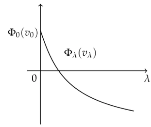
The following pictures give the possible graphs of the fiber maps.

φv

0 t

t(v)

a)

φv

0 t(v) t b) Figure 2.1: Possible graphs of the fiber maps.

Motivated by [25], we define the following constraint sets N₁ =

v ∈V+:kvk²−

Z

Ω f(x,g(v))g⁰(v)v≥

Z

Ωh(x)(g(v))^−γg⁰(v)v

and

N₂=

v∈V+:kvk²−

Z

Ω f(x,g(v))g⁰(v)v=

Z

Ωh(x)(g(v))^−γg⁰(v)v

. Observe that ifvis a solution of (P_A) thenv∈ N_2andN₂ ⊂ N_1.

It should be noted that forγ>1,N₂ is not closed as usual (certainly not weakly closed).

We prove that every function in D+(J) may be projected on the set N₂. In particular, N₁6=_∅.

Lemma 2.5. For any v∈D+(J)we have t(v)v∈ N₂.

Proof. From Lemma2.4we infer thatt(v)is a global minimum ofφ_vand hence, by Lemma2.3 one hasφ⁰_v(t(v)) =0. Thus

0=t(v)φ⁰_v(t(v))

=kt(v)vk²−

Z

Ωh(x)(g(t(v)v))^−γg⁰(t(v)v)(t(v)v)−

Z

Ω f(x,t(v)v)g⁰(t(v)v)(t(v)v) =0, namely,t(v)v∈ N₂⊂ N₁. The proof is complete.

We end this section with the following lemmas, which will be used to prove the regularity of the solutions.

Lemma 2.6. Let Ω be a bounded domain in R^N with smooth boundary ∂Ω. Let u ∈ L¹_loc(_Ω)and assume that, for some k≥0, u satisfies, in the sense of distributions,

(−_∆u+ku≥0 inΩ

u≥0 inΩ.

Then either u≡0, or there existse>0such that u(x)≥ ed(x,∂Ω), x∈ _Ω.

Proof. See Brezis–Nirenberg [3, Theorem 3].

Lemma 2.7. Let a ∈ L¹(_Ω)and suppose that there exist constants δ ∈ (0, 1)and C > 0 such that

|a(x)| ≤Cφ⁻₁^δ(x)_,for a.e. x∈ _Ω. Then, the problem (−_∆u =a inΩ

u=0 on∂Ω,

has a unique solution u∈ H₀¹(_Ω). Furthermore, there exist constantsα∈(0, 1)and M>0depending only on C,α,Ωsuch that u∈C^1,α(_Ω)and|u|_1,α < M.

Proof. See Hai [11, Lemma 2.1, Remark 2.2].

Remark 2.8. For future use we recall that there exist constantsl₁,l₂ >0 such that l₁d(x,∂Ω)≤φ₁(x)≤ l₂d(x,∂Ω)_, x∈ _Ω,

whereφ₁ is the first eigenfunction of(−_∆,H₀¹(_Ω)).

Lemma 2.9. Letψ_j: Ω×(0,∞)−→[0,∞),j=1, 2are measurable functions such that ψ₁(x,s)≤ψ₂(x,s) for all(x,s)∈_Ω×(_0,∞)_,

and for each x ∈ Ω, the function s 7−→ ψ₁(x,s)s⁻¹ is decreasing on (0,∞). Furthermore let u,v ∈ H¹(_Ω), with u∈ L^∞(_Ω)_,u>_0,v>₀onΩare such that

−_∆u≤ ψ₁(x,u) and −_∆v≥ψ₂(x,v) on Ω.

If u≤ v on∂Ωandψ₁(·,u)(orψ₂(·,u)) belongs to L¹(_Ω), then u≤v onΩ.

Proof. See Mohammed [20, Theorem 4.1].

3 Proof of Theorem 1.1

In this section, we shall prove Theorem 1.1. First, we shall show the existence of a global minimum of ΦonN₁. For this purpose, we need the following lemma.

Lemma 3.1. The setN₁is not empty and the functionalΦis coercive onN₁.

Proof. Since (1.7) holds, Lemmas2.2and2.5 implyN₁ 6=∅. We now show thatΦis coercive on N₁. Indeed, for everyv∈ N₁,

Φ(v) = ¹ 2

Z

Ω|∇v|²+ ¹ γ−1

Z

Ωh(x)(g(v))^1−γ− ¹ p+1

Z

Ωb(x)(g(v))^p+1

≥ ¹ 2

Z

Ω|∇v|²− kbk_∞ p+1

Z

Ω(g(v))^p+1,

and from Lemma2.1 (5)and Sobolev embedding we obtain Φ(v)≥ ¹

2 Z

Ω|∇v|²− kbk_∞ p+1

Z

Ω|v|^p+1≥ kvk²

2 −Ckvk^p+1 p+1 , for some constantC>0. Since p∈(0, 1)one infers thatΦis coercive onN₁.

As an immediate consequence of Lemma3.1, we can deduce that J₁= inf

v∈N₁Φ(v) and J₂ = inf

v∈N₂Φ(v) are well defined with J₁,J₂∈_Rand J₂ ≥ J₁.

We now prove that the infimum ofΦonN₁ is attained.

Lemma 3.2. There exists v∈ N₂such that J₁ =_Φ(v) =J2.

Proof. Let{v_n} ⊂ N₁be a minimizing sequence for Φ. From Lemma3.1the sequence{v_n} ⊂ N₁is bounded and then, up to subsequences, there existsv ∈ H₀¹(_Ω)_{such that}











v_n*v in H₀¹(_Ω),

v_n−→v in L^s(_Ω)for alls∈ (0, 2^∗), v_n−→v a.e. inΩ.

Sincev_n >_{0 a.e. in Ω, we have}v ≥_{0 a.e. in}Ω, that is, v∈ V+. From the definition of N₁ and Lemma2.1 (3),(4),(5)it follows that for some constantCone has

1 2

Z

Ωh(x)(g(v_n))^1−γ ≤

Z

Ωh(x)(g(v_n))^−γg⁰(v_n)v_n

≤ kvnk²−

Z

Ωb(x)(g(vn))^pg⁰(vn)vn

≤ kv_nk²+

Z

Ω|b(x)||v_n|^p+1

≤ kv_nk²+c||v_n||^p+1

≤C.

Therefore, using Fatou’s lemma we getR

Ωθ(x)≤ C<_{∞, where} θ(x) =

(h(x)(g(v(x)))^1−γ, if v(x)6=0

∞, if v(x) =0.

Since g(0) = 0 (by Lemma 2.1 (2)) and R

Ωθ(x) < ∞, it follows that v > 0 a.e. inΩ. Thus, using Fatou’s lemma again, we obtain

0<

Z

Ωh(x)(g(v))^−γg⁰(v)v≤C

and this jointly with Lemma2.2imply thatv∈ D+(J). As a consequence, Lemmas2.4and2.5 apply yielding a global minimumt(v)> 0 such that φ_v(t(v)) =inf_t>0φ_v(t)andt(v)v ∈ N₂. Furthermore, we have

J₁ = lim

n→_∞Φ(v_n) =lim inf

n→_∞ Φ(v_n)

=lim inf

n→_∞

1 2

Z

Ω|∇v_n|²+ ¹ γ−1

Z

Ωh(x)g(v_n)^1−γ− ¹ p+1

Z

Ωb(x)(g(v_n))^p+1

≥lim inf

n→_∞

1 2

Z

Ω|∇vn|²

+lim inf

n→_∞

1 γ−1

Z

Ωh(x)(g(vn))^1−γ

− ¹ p+1

Z

Ωb(x)(g(v))^p+1

≥ ¹ 2

Z

Ω|∇v|²+ ¹ γ−1

Z

Ωh(x)(g(v))^1−γ− ¹ p+1

Z

Ωb(x)(g(v))^p+1 =φ_v(1)

≥φv(t(v)) =_Φ(t(v)v)

≥ J₂

≥ J₁. Hence

J₁ =φ_v(1) =_Φ(v) =J₂,

that is,φv(1) =φv(t(v)) =inft>₀φv(t). This impliesφ_v⁰(1) =0 and consequentlyv∈ N₂ ⊂ N₁.

We are now ready to prove Theorem1.1.

Proof of Theorem1.1. a)Necessity.Suppose thatu∈ H₀¹(_Ω)is a solution of (P), by taking ϕ= u in (1.1), we have

Z

Ωh(x)|u|^1−γ <_∞.

Sufficiency. Let v be the global minimum obtained in Lemma 3.2. We will prove that v is a solution of (P_A). Let ϕ∈ H₀¹(_Ω)_, ϕ≥0. Applying Lemma2.1 (₁₀)_{we find}

Z

Ωh(x)(g(v+eϕ))^1−γ ≤

Z

Ωh(x)(g(v))^1−γ <_∞ ∀e>0,

namely,v+eϕ ∈D+(J)_{for every}e>0. Then, from Lemmas2.4and2.5there exists at(e)>₀ such thatφv+eϕ(t(e)) =inft>₀φv+eϕ(t)andt(e)(v+eϕ)∈ N₂. Therefore

Φ(v+eϕ) =φ_v+eϕ(₁)≥φ_v+eϕ(t(e)) =_Φ(t(e)(v+eϕ))≥ J₂ =_Φ(v)_,

that is,

Z

Ω

h(x)(g(v+eϕ))^1−γ−h(x)(g(v))^1−γ 1−γ

≤ kv+eϕk²− kvk²

2 −

Z

Ω

b(x)(g(v+eϕ))^p+1−b(x)(g(v))^p+1

p+1 .

Thus, dividing both sides of the above inequality by e > 0, passing to the limit inferior as e−→0 and using Fatou’s Lemma, we have

Z

Ωh(x)(g(v))^−γg⁰(v)ϕ=

Z

Ωlim infh(x)(g(v+eϕ))^1−γ−h(x)(g(v))^1−γ 1−γ

≤

Z

Ω∇v∇ϕ−

Z

Ωb(x)(g(v))^pg⁰(v)ϕ. (3.1) Finally, we can use an argument inspired by Graham–Eagle [10] to show thatvis a solution of (P_A). Since v∈ N₂, one has

kvk²−

Z

Ωb(x)(g(v))^pg⁰(v)v−

Z

Ωh(x)(g(v))^−γg⁰(v)v=0.

For arbitraryϕ∈ H₀¹(_Ω)ande>0, setΨ= (v+eϕ)⁺and

Ω^e₁={x∈_Ω:b(x)<0 andv(x) +eϕ(x)<0}. Then, insertingΨ into (3.1) and usingv∈ N₂, we obtain that

0≤

Z

Ω∇v∇_Ψ−

Z

Ωb(x)(g(v))^pg⁰(v)_Ψ−

Z

Ωh(x)(g(v))^−γg⁰(v)_Ψ

=

Z

[v+eϕ≥0]

∇v∇(v+eϕ)−b(x)(g(v))^pg⁰(v)(v+eϕ)−h(x)(g(v))^−γg⁰(v)(v+eϕ)

= _Z

Ω−

Z

[v+eϕ<0]

∇v∇(v+eϕ)−b(x)(g(v))^pg⁰(v)(v+eϕ)−h(x)(g(v))^−γg⁰(v)(v+eϕ)

=kvk²−

Z

Ωb(x)(g(v))^pg⁰(v)v−

Z

Ωh(x)(g(v))^−γg⁰(v)v +e

_Z

Ω∇v∇ϕ−b(x)(g(v))^pg⁰(v)ϕ−h(x)(g(v))^−γg⁰(v)ϕ

−

Z

[v+eϕ<₀]

∇v∇(v+eϕ)−b(x)(g(v))^pg⁰(v)(v+eϕ)−h(x)(g(v))^−γg⁰(v)(v+eϕ)

≤e _Z

Ω∇v∇ϕ−b(x)(g(v))^pg⁰(v)ϕ−h(x)(g(u))^−γg⁰(v)ϕ

−e Z

[v+eϕ<0]

∇v∇ϕ+e Z

Ω^e₁b(x)(g(v))^pg⁰(v)ϕ.

Since the measure of the domains of integration[v+eϕ <₀]andΩ^e₁ tends to zero ase →0, we then divide the above expression bye>0 to obtain

0≤

Z

Ω∇v∇ϕ−b(x)(g(v))^pg⁰(v)ϕ−h(x)(g(v))^−γg⁰(v)ϕ, ase→0. Replacing ϕby−ϕwe conclude:

Z

Ω∇v∇ϕ−b(x)(g(v))^pg⁰(v)ϕ−h(x)(g(v))^−γg⁰(v)ϕ=0, ∀ϕ∈ H₀¹(_Ω),

and thereforev is a solution of (P_A). This means thatu = g(v) is a solution of problem (P).

We complete the proof ofa).

b)Suppose that vis a solution of (P_A). We will show thatv ∈ C^1,α(_Ω)and hence, asg ∈ C^∞ we getu= g(v)∈C^1,α(_Ω). Sincev6≡0 satisfies in the sense of distributions

(−_∆v≥0 inΩ, v≥0 inΩ, we can apply Lemma2.6yielding ae>0 such that

v(x)≥ed(x,∂Ω), x∈_Ω,

ed(x,∂Ω)<1, x∈ _Ω. (3.2)

Then, by (1.8) and Lemma 2.1 (3),(8),(10) there exist constants c,C > 0 and β ∈ (0, 1) such that

|h(x)(g(v))^−γg⁰(v)| ≤h(x)(g(ed(x,∂Ω)))^−γ ≤ h(x)C(ed(x,∂Ω))^−γ

≤Ccd^γ−β(x,∂Ω)d^−γ(x,∂Ω)

=Cd^−β(x,∂Ω)

≤Cφ⁻₁^β(x) _(3.3)

for every x ∈ _Ω, and hence h(g(v))^−γg⁰(v) ∈ L¹(_Ω). Thus, by Lemma 2.7 there exists a solutionΨ1 ∈C^1,α1(_Ω), for someα₁ ∈(0, 1), of the problem











−_∆w= h(x)(g(v))^−γg⁰(v) inΩ,

w>0 inΩ,

w=0 on∂Ω.

Next, we prove that the problem











−_∆w=b(x)(g(v))^pg⁰(v) in Ω,

w>0 in Ω,

w=0 on ∂Ω,

(3.4)

has a unique solutionΨ2 ∈C^1,α2(_Ω)_{, for some}α₂ ∈(_{0, 1})_.

Letδ :=1−p ∈(0, 1). From (3.2) and Lemma2.1(8),(12)we have

|b(x)g^p(v(x))g⁰(v(x))| ≤ kbk_∞g^−δ(v(x))(g(v(x))g⁰(v(x)))≤ Cφ₁^−δ(x), that is,

|b(x)g^p(v(x))g⁰(v(x))| ≤Cφ₁^−δ(x),

for every x ∈ _Ω and some constant C > 0. Therefore, by Lemma 2.7 problem (3.4) has a unique solutionΨ2∈ C^1,α2(_Ω), for someα₂∈ (0, 1).

We claim thatv=_Ψ1+_Ψ2. Indeed, using the fact thatΨ1,Ψ2 andvare solutions, we find Z

Ω∇v∇ϕ=

Z

Ω

h(x)(g(v))^−γg⁰(v) +b(x)(g(v))^pg⁰(v)ϕ=

Z

Ω∇(_Ψ1+_Ψ2)∇ϕ,

for everyϕ∈ H₀¹(_Ω). Therefore,v=_Ψ1+_Ψ2, and thenv∈C^1,α(_Ω), whereα:=min{α₁,α₂} ∈ (0, 1). Thus, the claim follows, and consequentlyu = g(v) ∈ C^1,α(_Ω) showing the regularity of the solutions of (P).

Finally, we show the uniqueness of solution to (P). For this purpose, we show the unique- ness of solution to (P_A). Let v₁ andv₂ be two solutions of (P_A). We will prove thatv₁ ≤v₂in Ω. First, let us set

j(x,s):=h(x)(g(s))^−γg⁰(s) +b(x)(g(s))^pg⁰(s).

Fix x ∈ Ω. According to Lemma2.1 (9),(10),(11), the functions 7−→ j(x,s)s⁻¹ is decreasing on (0,∞). Moreover, from (3.3) one has

0≤ j(x,v_i)≤Cφ₁^−β(x) +b(x)(g(v_i(x)))^pg⁰(v_i(x)), x∈_Ω,

hence j(x,v_i)∈ L¹(_Ω)fori= 1, 2. Thus, we can use Lemma2.9 withψ_i = j(i=1, 2),u = v₁ and v= v2 to getv₁ ≤ v2 in Ω. Similarly we get v2 ≤ v₁ in Ω, thus v₁ = v2. This concludes the proof of the theorem.

Remark 3.3. If (1.8) holds, then problem (P) has a solution. Indeed, choosev₀=φ₁∈ H₀¹(_Ω). From Remark 2.8 and (1.8) we have h|φ₁|^1−γ ≤ cl₁^β−γ|φ₁|^1−β ∈ L¹(_Ω). Theorem 1.1 a)then guarantees the existence of a solution of (P).

4 Proof of Theorem 1.3

In this section, we assume (f)₂, that is, f(x,s) = −b(x)s^22∗−1 with 0 ≤b∈ L^∞(_Ω)andb6≡0.

Since the embedding H₀¹(_Ω) ,→ L^2∗(_Ω) is not compact, the proof of Lemma 3.2 can not be applied directly here. In order to overcome this difficulty, we use the Brezis–Lieb Theorem (see [2]).

Now, we have Φ(_v) = ¹

2 Z

Ω|∇v|²+ ¹ γ−1

Z

Ωh(_x)(_g(_v))^1−γ+ ¹ 22^∗

Z

Ωb(_x)(_g(_v))^22∗_, forv∈ D(J). From (1.7) and Lemmas2.2and2.5, one hasN₁ 6=_∅.

We will show the following.

Lemma 4.1. The functionalΦis coercive onN₁

Proof. For everyv∈ N_{1, we haveΦ}(v)≥ ¹₂kvk²_{and hence,Φ}is coercive on N_1. As an immediate consequence of Lemma4.1, we can deduce that

J₁= inf

v∈N₁Φ(v) and J₂ = inf

v∈N₂Φ(v) are well defined with J₁,J₂∈_Rand J₂ ≥ J₁.

Next, we prove the following lemma.

Lemma 4.2. There exists v∈ N₂such that J₁ =_Φ(v) =J₂.

Proof. Let{v_n} ⊂ N₁ be a minimizing sequence forΦ. From Lemma4.1the sequence{v_n} ⊂ N₁ is bounded in H₀¹(_Ω), so in L^2∗(_Ω) too, and then, up to subsequences, there exists v ∈ H₀¹(_Ω)such that











v_n*v inH₀¹(_Ω),

v_n−→v inL^s(_Ω)for alls ∈(0, 2^∗), vn−→v a.s. inΩ.

As a consequence, by Lemma2.1(6), there exists a constantC>0 such that Z

Ωb(x)(g(vn))^22∗ =

Z

Ω

h

b^21∗i2^∗

(g(vn))²²

∗

≤ kbk_∞K₀^22∗ Z

Ω|vn|^2∗ ≤C.

Moreover, b(x)(g(v_n))^22∗ −→ b(x)(g(v))^22∗ _{a.s. in} Ω. Hence, by virtue of the Brezis–Lieb Theorem (see [2]) it follows that

Z

Ωb(x)(g(v_n))^22∗ =

Z

Ωb(x)(g(v))^22∗+

Z

Ωb(x)|(g(v_n))^22∗−(g(v))^22∗|+o(1)

≥

Z

Ωb(x)(g(v))^22∗+o(1).

(4.1)

We can repeat the arguments used in Lemma3.2to prove the following.

• v>0 a.e. inΩand Z

Ωh(x)(g(v))^−γg⁰(v)v< _∞;

• there existst(v)>0 such thatt(v)v∈ N₂. Then, by (4.1) and the Fatou’s lemma we find

J₁ =limΦ(v_n)

=lim inf 1

2 Z

Ω|∇v_n|²+ ¹ γ−1

Z

Ωh(x)(g(v_n))^1−γ+ ¹ 22^∗

Z

Ωb(x)(g(v_n))^22∗

≥ ¹ 2

Z

Ω|∇v|²+ ¹ γ−1

Z

Ωh(x)(g(v))^1−γ+ ¹ 22^∗

Z

Ωb(x)(g(v))^22∗

=φ_v(1)

≥φv(t(v)) =_Φ(t(v)v)≥ J₂ ≥ J₁. Hence

J₁ =φ_v(1) =_Φ(v) =J₂,

that is,φ_v(1) =φ_v(t(v)) =inf_t>0φ_v(t). This impliesφ_v⁰(1) =0 and consequentlyv∈ N₂ ⊂ N₁. This ends the proof.

We are now ready to prove Theorem1.3.

Proof of Theorem1.3. Necessity. Repeating the argument used to prove the corresponding claim in Theorem1.1 a), the result follows.

Sufficiency. Let v be the global minimum obtained in Lemma 4.2. We will prove that v is a solution of (P_A). Let ϕ ∈ H₀¹(_Ω), ϕ ≥ 0 and e > 0. We can repeat the arguments used in Theorem1.1 a)to prove the following.

• h(·)(g(v+eϕ))^1−γ ∈ L¹(_Ω)_;