HAT-P-68b: A TRANSITING HOT JUPITER AROUND A K5 DWARF STAR ∗

(1)

Typeset using L^ATEXtwocolumnstyle in AASTeX61

HAT-P-68b: A TRANSITING HOT JUPITER AROUND A K5 DWARF STAR ^∗

Bethlee M. Lindor,^{1, 2, 3} Joel D. Hartman,³ Gáspár Á. Bakos,^{3, 4,}^† Waqas Bhatti,³ Zoltan Csubry,³ ⁵ Kaloyan Penev,⁵ Allyson Bieryla,⁶ David W. Latham,⁶ Guillermo Torres,⁶Lars A. Buchhave,⁷ Géza Kovács,⁸

Miguel de Val-Borro,⁹ Andrew W. Howard,¹⁰ Howard Isaacson,¹¹Benjamin J. Fulton,^{10, 12}Isabelle Boisse,¹³ Alexandre Santerne,¹⁴ Guillame Hébrard,¹⁵ Támás Kovács,⁸Chelsea X. Huang,¹⁶Jack Dembicky,¹⁷ Emilio Falco,⁶ Bence Béky,¹⁸ Mark E. Everett,¹⁹ Elliott P. Horch,²⁰ József Lázár,²¹ István Papp,²¹ and

P´al S´ari²¹ ¹⁰

1Astronomy Department, University of Washington, Seattle, WA 98195, USA

2NSF Graduate Student Research Fellow

3Department of Astrophysical Sciences, Princeton University, NJ 08544, USA

4MTA Distinguished Guest Fellow, Konkoly Observatory, Hungary

5Department of Physics, University of Texas at Dallas, Richardson, TX 75080, USA ¹⁵

6Harvard-Smithsonian Center for Astrophysics, 60 Garden St, Cambridge, MA 02138, USA

7Centre for Star and Planet Formation, Natural History Museum of Denmark, University of Copenhagen, DK-1350 Copenhagen, Denmark

8Konkoly Observatory of the Hungarian Academy of Sciences, Budapest, Hungary

9Astrochemistry Laboratory, Goddard Space Flight Center, NASA, 8800 Greenbelt Rd, Greenbelt, MD 20771, USA

10Department of Astronomy, California Institute of Technology, Pasadena, CA, USA ²⁰

11Department of Astronomy, University of California, Berkeley, CA, USA

12IPAC-NASA Exoplanet Science Institute, Pasadena, CA, USA

13Aix Marseille Universit´e, CNRS, LAM (Laboratoire d’Astrophysique de Marseille) UMR 7326, F-13388, Marseille, France

14Instituto de Astrofisica e Ciˆencias do Espa¸co, Universidade do Porto, CAUP, Rua das Estrelas, PT4150-762 Porto, Portugal

15Institut d’Astrophysique de Paris, UMR7095 CNRS, Universit´e Pierre & Marie Curie, 98bis boulevard Arago, 75014 Paris, France ²⁵

16Department of Physics, and Kavli Institute for Astrophysics and Space Research, Massachusetts Institute of Technology, Cambridge, MA 02139, USA

17Apache Point Observatory, Sunspot, NM 88349, USA

18Google, Googleplex, 1600 Amphitheatre Parkway, Mountain View, CA 94043, USA

19National Optical Astronomy Observatory, Tucson, AZ, USA ³⁰

20Department of Physics, Southern Connecticut State University, 501 Crescent Street, New Haven, CT 06515, USA

21Hungarian Astronomical Association, 1451 Budapest, Hungary

ABSTRACT

We report the discovery by the ground-based HATNet survey of the transiting exoplanet HAT-P-68b, which has a mass of 0.724±0.043MJ, and radius of 1.072±0.012RJ. The planet is in a circular P = 2.2984 -day orbit around a ³⁵ moderately bright V = 13.937±0.030 magnitude K dwarf star of mass 0.673^+0.020₋_0.014M_⊙, and radius 0.6726±0.0069R_⊙. The planetary nature of this system is confirmed through follow-up transit photometry obtained with the FLWO 1.2 m telescope, high-precision RVs measured using Keck-I/HIRES, FLWO 1.5 m/TRES, and OHP 1.9 m/Sophie, and high- spatial-resolution speckle imaging from WIYN 3.5 m/DSSI. HAT-P-68 is at an ecliptic latitude of +3^◦ and outside the field of view of both the NASA TESSprimary mission and the K2mission. The large transit depth of 0.036 mag ⁴⁰ (r-band) makes HAT-P-68b a promising target for atmospheric characterization via transmission spectroscopy.

Corresponding author: Bethlee M. Lindor blindor@uw.edu

∗Based on observations obtained with the Hungarian-made Automated Telescope Network. Based in part on observations made with the Keck-I telescope at Mauna Kea Observatory, HI (Keck time awarded through NASA programs N133Hr and N169Hr). Based in part on observations obtained with the Tillinghast Reflector 1.5 m telescope and the 1.2 m telescope, both operated by the Smithsonian Astrophysical Observatory at the Fred Lawrence Whipple Observatory in Arizona. Based on radial velocities obtained with the Sophie spectrograph mounted on the 1.93 m telescope at Observatoire de Haute-Provence.

(2)

Keywords: planetary systems — stars: individual ( HAT-P-68, GSC 1925-01046 ) techniques: spectroscopic, photometric

†Packard Fellow

(3)

1. INTRODUCTION

The first detection of a planet orbiting a star besides ⁴⁵ our own (Mayor & Queloz 1995) sparked a new era of astronomy and planetary science, and made the discovery and characterization of extra-solar planets a focal point of observational research in astrophysics. Among the various methods available, transit photometry has ⁵⁰ produced the largest yield of exoplanets to date, and has also proven to be the most sensitive method for dis- covering small planets¹. Additionally, transiting exoplanets (TEPs) offer the unique opportunity to study the physical properties of planets outside the Solar Sys- ⁵⁵ tem, and how these properties depend on those of their parent stars. Combining transit time-series data with measurements of the radial velocity (RV) orbital wob- ble of the host star provides the masses and radii of planetary objects – that is, if the stellar mass and ra- ⁶⁰ dius can be determined through other means. Further- more, follow-up observations of these systems allow us to study the structure and composition of the planetary atmospheres through transmission spectroscopy (e.g. Charbonneau et al. 2002), and to measure the or- ⁶⁵ bital eccentricity and obliquity (e.g. Morton & Winn 2014). These capabilities make TEPs one of the most reliable sources for testing current models of planetary formation and evolution.

Many wide-field ground-based surveys have been ⁷⁰ productive in detecting TEPs, including HATNet (Bakos et al. 2004), HATSouth (Bakos et al. 2013), and WASP (Pollacco et al. 2006). The sample of exoplanets discovered by these surveys is highly biased towards giant planets at short orbital distances to their host ⁷⁵ stars (e.g.Gaudi et al. 2005). These hot Jupiters (HJs) initially shattered our understanding of planetary formation. Space surveys like the all-sky Transiting Ex- oplanet Survey Satellite (TESS; Ricker et al. 2014) – joining the legacy of Kepler (Borucki et al. 2010), K2 ⁸⁰ (Howell et al. 2014), and CoRot (Auvergne et al. 2009) – are better equiped to identify objects with a wider range of sizes at a wide range of orbital distances to their host stars.

Yet, discoveries of planets with orbital periods ⁸⁵ shorter than 10 days provide advantages to resolv- ing current theoretical challenges in the field (see Dawson & Johnson 2018). For instance, explaining the inflated radii of hot Jupiters remains a theoretical puz- zle (e.g. Sestovic et al. 2018, and references therein) ⁹⁰ that may be elucidated by building up a larger sample

1 NASA Exoplanet Archive accessed Feb. 2020;

http://exoplanetarchive.ipac.caltech.edu

objects to disentangle the effects of age, orbital separation, irradiation, composition and mass on the radii of these planets (e.g., Hartman et al. 2016). Explain- ing the origin of these planets is another open problem ⁹⁵ (Dawson & Johnson 2018, e.g.,) that can be better ad- dressed with a larger sample of objects.

The HATNet survey searches for planets transiting moderately bright stars by utilizing six small telephoto lenses on robotic mounts. Specifically, HATNet has two ¹⁰⁰ stations with multiple 11 cm telescopes; one of which is located at the Smithsonian Astrophysical Observatory’s Fred Lawrence Whipple Observatory (FLWO) in Ari- zona, while the other is atop the Mauna Kea Observa- tory (MKO) in Hawaii. Bakos (2018) provides a recent ¹⁰⁵ review of the HATNet and HATSouth projects.

Here we present the discovery by the HATNet survey of a transiting, short-period, gas-giant planet around a K dwarf star. Section 2 summarizes the observational data that led to the discovery, as well as various follow- ¹¹⁰ up studies performed for HAT-P-68. This involved photometric and spectroscopic observations, and high resolution imaging. In Section 3, we analyze the data to rule out false positive scenarios and determine the best- fit stellar and planetary parameters. We discuss our ¹¹⁵ results in Section4.

2. OBSERVATIONS

We have used a number of observations to aid our understanding of HAT-P-68, and to confirm the exis- tence of an extra-solar planet in the system. These ¹²⁰ observations include discovery light curves obtained by the HATNet survey, ground-based follow-up transit light curves, high-resolution spectra and associated RVs, high-spatial resolution imaging, and catalog broad-band photometry and astrometry. We describe the observa- ¹²⁵ tions collected by our team in the following sections.

See Tables 1 and3 for brief summaries of all the spectroscopic and photometric observations collected for HAT-P-68.

2.1. Photometric Detection ¹³⁰ Observations of a field containing HAT-P-68 were carried out between 2011 November and 2012 May by the HAT-5 and HAT-8 instruments located at FLWO and MKO, respectively. A total of 5867 and 3034 exposures of 3 minutes were obtained with each de- ¹³⁵ vice through a Sloan r filter, after which the images were reduced to trend-filtered light curves following Bakos et al. (2010). Here we used the Trend-Filtering Algorithm (TFA;Kov´acs et al. 2005) in signal-detection mode. The final point-to-point precision for the HAT- ¹⁴⁰ Net light curve of HAT-P-68 is 2.4%.

(4)

-0.06 -0.04 -0.02 0 0.02 0.04 0.06

-0.4 -0.2 0 0.2 0.4

∆ mag

Orbital phase HAT-P-68 HATNet Light Curve

-0.06 -0.04 -0.02 0 0.02 0.04 0.06

-0.04 -0.02 0 0.02 0.04

∆ mag

Orbital phase

-0.06 -0.04 -0.02 0 0.02 0.04 0.06

-0.04 -0.02 0 0.02 0.04

∆ mag

Orbital phase

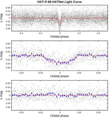
Figure 1. Discovery HATNet transit light curve phase- folded with a period of 2.2984 daysTop: The full unbinned instrumentalr band light curve. The gray points show the individual measurements, while the solid red line shows the best-fit transit model. Middle: Same as the top panel, here we restrict the horizontal range of the plot to better dis- play the transit. The filled blue circles show the light curve averaged in phase using a bin-size of 0.002. Bottom: The residuals from the best-fit transit model.

We searched the light curves from the aforemen- tioned field for periodic box-shaped transit events using the Box Least Squares method (BLS;Kov´acs et al.

2002), and detected 3.6% deep transits with a period of

145

2.2984 days in the light curve of HAT-P-68. This detection prompted additional photometric and spectroscopic follow-up observations, as described in the subsections below. Figure 1 shows the HATNet light curve phase folded at the period identified with BLS, together with

150

our best-fit transit model. The differential photometry data are made available in Table4.

After subtracting the best-fit primary transit model from the HATNet light curve, we used BLS to search the residuals for additional periodic transit signals. No

155

other significant transit signals were identified. We can place an approximate upper limit of 1% on the depth of any other periodic transit signals in the light curve with periods shorter than∼10 days.

To supplement the search for periodic transit sig-

160

nals, we also searched the HATNet light curve residuals

0 0.001 0.002 0.003 0.004 0.005 0.006 0.007 0.008 0.009

10 20 30 40 50 60 70 80 90 100 FAP = 10^-5

GLS Unnormalized Periodgram

Period [days]

HAT-P-68 - HATNet Photometric Rotation Period

-0.1 -0.08 -0.06 -0.04 -0.02 0 0.02 0.04 0.06 0.08

0 0.1 0.2 0.3 0.4 0.5 0.6 0.7 0.8 0.9 1

∆Mag

Phase

-0.015 -0.01 -0.005 0 0.005 0.01 0.015

0 0.1 0.2 0.3 0.4 0.5 0.6 0.7 0.8 0.9 1

∆Mag

Phase

Figure 2. Detection of a P = 24.593±0.064 days photometric rotation period signal in the HATNet light curve of HAT-P-68. Top: The Generalized Lomb-Scargle (GLS) periodogram of the HATNet light curve after subtracting the best-fit transit model. The horizontal blue line shows a bootstrap-calibrated 10⁻⁵ false alarm probability (FAP) level. Middle: The HATNet light curve phase-folded at the peak GLS period. The gray points show the individual photometric measurements, while the dark red filled squares show the observations binned in phase with a bin size of 0.02. Bottom: Same as the middle panel, here we restrict the vertical range of the plot to better show the variation seen in the phase-binned measurements.

for sinusoidal periodic variations using the Generalized Lomb-Scargle (GLS) periodogram (Zechmeister & K¨urster 2009). This search detected a P = 24.593±0.064 day periodic quasi-sinusoidal signal, from which we com-

165

puted a bootstrap-calibrated false alarm probability of

(5)

10⁻^10.3 and a periodogram signal-to-noise ratio of 36 as described in Hartman & Bakos (2016). The GLS periodogram and phase-folded light curve are shown in Figure 2. We provisionally identify this as the pho- ¹⁷⁰ tometric rotation period of the star, and note that the period and amplitude are in line with other mid K dwarf main sequence stars (e.g.,Hartman et al. 2011).

2.2. Reconnaissance Spectroscopy

Initial reconnaissance spectroscopy observations of ¹⁷⁵ HAT-P-68 were obtained using the Astrophysical Re- search Consortium Echelle Spectrometer (ARCES;

Wang et al. 2003) on the ARC 3.5 m telescope located at Apache Point Observatory (APO) in New Mexico. Us- ing this facility, we obtained three ∆λ/λ≡R= 18,000 ¹⁸⁰ resolution spectra of HAT-P-68 on UT 2012 Oct 30, 2012 Nov 7, and 2013 Mar 3. These had exposure times of 3600 s, 2740 s, and 2740 s, respectively, yielding signal-to-noise ratios per resolution element near 5180 ˚A of 32.3, 25.6, and 26.8, respectively. The ´echelle images ¹⁸⁵ were reduced to wavelength-calibrated spectra following Hartman et al.(2015).

We applied the Stellar Parameter Classification (SPC;

Buchhave et al. 2012) method on the ´echelle images to measure the RV and atmospheric parameters for the ¹⁹⁰ stellar host. In particular, this pipeline derives the effective temperature (Teff⋆), surface gravity (logg), metallicity ([Fe/H]) and projected equatorial rotation velocity (vsini). Based on the three ARCES observations we es- timatedTeff⋆ = 4500±50 K, logg = 4.62±0.10 (cgs), ¹⁹⁵ [Fe/H] = −0.14±0.08 and vsini = 2.5±0.5 km s⁻¹. We caution that the uncertainties based on this analysis are likely underestimated compared to the values reported in Section3.1based on an SPC analysis of Keck- I/HIRES observations. The three RV measurements ²⁰⁰ were consistent with no variation, with a mean value of

−8.69 km s⁻¹, and a standard deviation of 0.43 km s⁻¹, comparable to the systematic uncertainties in the wavelength calibration. We note that the cross-correlation functions were consistent with a single K dwarf star, ²⁰⁵ with no evidence of a second set of absorption lines present in the spectra.

2.3. High RV-Precision Spectroscopy

Following the reconnaissance, we obtained higher resolution, and higher RV-precision spectroscopic observa- ²¹⁰ tions of HAT-P-68 to further characterize it. To carry out these observations we used the Tillinghast Reflec- tor Echelle Spectrograph (TRES; F˝uresz 2008) on the 1.5 m Tillinghast Reflector at FLWO, the Sophie spectrograph (Bouchy et al. 2009) on the Observatoire de ²¹⁵ Haute Provence (OHP) 1.93 m in France, and HIRES

-200 -150 -100 -50 0 50 100 150 200

RV (ms-1)

HAT-P-68 RVs and BSs HIRES

TRES Sophie

-80-60 -40-20 20 40 60 80 0 100 120 140

O-C (ms-1)

-5000 0 5000 10000 15000 20000 25000 30000

0.0 0.2 0.4 0.6 0.8 1.0

BS (ms-1)

Phase with respect to T_c

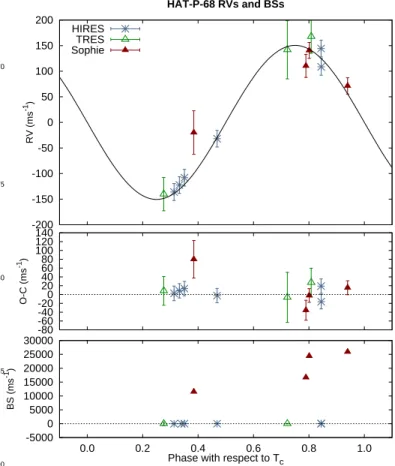
Figure 3. Top: High-precision RV measurements from FLWO 1.5 m/TRES, OHP 1.9 m/Sophie, and Keck- I 10 m/HIRES, together with our best-fit orbit model, plotted as a function of orbital phase. Phase zero corresponds to the time of mid transit. The center-of-mass velocity has been subtracted. The error bars include the jitter which is varied independently for each instrument in the fit. Middle: RV O−Cresiduals from the best-fit model, plotted as a function of phase. Bottom: Spectral line bisector spans (BSs) plotted as a function of phase. Note the different vertical scales of the three panels.

(Vogt et al. 1994) on the Keck-I 10 m at MKO together with its I2absorption cell. The measured RVs and spectral line bisector spans (BSs) from these three facilities are provided in Table2and plotted in Figure3. ²²⁰

A total of 3 TRES spectra were obtained on UT 2012 Nov 23, 2013 Mar 1, and 2013 Oct 11 at a resolution of R= 44,000 and were reduced to high precision RVs and BSs followingBieryla et al. (2014), and to atmospheric

stellar parameters using SPC. ²²⁵

A total of four R = 39,000 spectra were obtained with Sophie on UT 2013 Oct 31, 2013 Nov 1, and 2013 Nov 6, and were reduced to high-precision RVs and BSs followingBoisse et al.(2013).

A total of six R = 55,000 spectra were obtained ²³⁰ through an I2 cell with HIRES on UT 2013 Oct 19,

(6)

0

0.05

0.1

0.15

0.2

0.25

-0.1 -0.05 0 0.05 0.1 0.15

∆ (mag) - Arbitrary offsets

Time from transit center (days) i-band

i

g

i

2013 Jan 3 - FLWO 1.2m

2013 Feb 16 - FLWO 1.2m

2016 Feb 22 - FLWO 1.2m

2016 Apr 1 - FLWO 1.2m

-0.1 -0.05 0 0.05 0.1 0.15

Time from transit center (days) HAT-P-68 Follow-up Light Curves

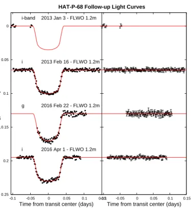
Figure 4. Unbinned folow-up transit light curves obtained with KeplerCam on the FLWO 1.2 m, plotted with the best- fit transit model as a solid red line. The dates of observation and photometric filters used are indicated. The residuals are shown on the right-hand side in the same order as the light curves.

2013 Dec 11–12, and 2015 Nov 26–28, while an I2- free template observation was obtained on UT 2013 Oct 19. These data were reduced to relative RVs following Butler et al. (1996), and to BSs following Torres et al.

235

(2007). We also applied SPC to the I2-free template to obtain high precision atmospheric parameters of the host star.

As seen in Figure3, the RVs from TRES, Sophie and HIRES exhibited a clear Keplerian orbital variation in

240

phase with the ephemeris from the photometric transits. We also find that the BSs from HIRES show al- most no variation. The TRES BS values had several hundred m s⁻¹uncertainties, and the Sophie values varied by many km s⁻¹, in both cases due to significant sky

245

contamination that affected the shapes of the CCFs.

2.4. Photometric Follow-up

In order to confirm the transit signal identified in the HATNet light curve of HAT-P-68, we carried out photometric follow-up observations of the system using the

250

KeplerCam mosaic CCD imager on the FLWO 1.2 m telescope. Observations used in the analysis were con- ducted on five nights covering four predicted primary

., Figure 5. Limits on the relative magnitude of a resolved companion to HAT-P-68 as a function of angular separation based on speckle imaging observations from WIYN 3.5 m/DSSI.Top: limits for the 692 nm filter. Bot- tom: limits for the 880 nm filter.

transit events, and one predicted secondary eclipse event. The nights, filters, number of exposures, effec-

255

tive cadences, and point-to-point photometric precision achieved are listed in Table 3. A sixth observation obtained on the night of 2013 Feb 10 did not observe either the primary transit or secondary eclipse, and was excluded from the analysis.

260

The KeplerCam CCD images were calibrated and reduced to light curves using the aperture photometry routine described by Bakos et al. (2010). We applied an External Parameter Decorrelation (EPD) and TFA- filtering of the light curves as part of the global modeling

265

of the system, which we discuss further in Section3. The four light curves covering the primary transit are shown in Figure4. The light curve covering the predicted secondary eclipse was consistent with no eclipse variation, and was used in the blend analysis of the system, but

270

was not included in the global analysis to determine the planetary and stellar parameters. All of the light curve data are made available in Table4.

2.5. Speckle Imaging

(7)

Table 1. Summary of Spectroscopic Observations

Telescope/Instrument UT Date(s) # Spectra Resolution S/N Range^a γRVb RV Precision^c

∆λ/λ (m s⁻¹) (m s⁻¹)

APO 3.5 m/ARCES 2012 Oct–2013 Mar 3 18000 26.8–32.3 −8690 430

FLWO 1.5 m/TRES 2012 Nov–2013 Nov 3 44000 10–17 −7930 16.8

OHP 1.9 m/Sophie 2013 Oct–Nov 4 39000 · · · −8892 48.6

Keck-I 10 m/HIRES 2013 Oct–2015 Nov 6 55000 81–115 · · · 12.5

a S/N per resolution element near 5180 ˚A. This was not measured for all of the instruments.

b For Sophie RV observations this is the zero-point RV from the best-fit orbit. For ARCES and TRES it is the mean value of the low-precision reconnaissance RV. Higher-precision RVs were measured from the TRES observations and used in the orbit fitting as well, however these are relative RV measurements that were not adjusted to an absolute standard.

c For high-precision RV observations included in the orbit determination this is the scatter in the RV residuals from the best-fit orbit (which may include astrophysical jitter), for other instruments this is either an estimate of the precision (not including jitter), or the measured standard deviation. We only provide this quantity when applicable.

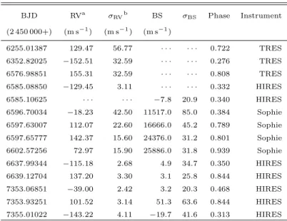
Table 2. Relative Radial Velocities and Bisector Spans of HAT- P-68.

BJD RV^a σRVb BS σBS Phase Instrument

(2 450 000+) (m s⁻¹) (m s⁻¹) (m s⁻¹)

6255.01387 129.47 56.77 · · · · · · 0.722 TRES

6352.82025 −152.51 32.59 · · · · · · 0.276 TRES

6576.98851 155.31 32.59 · · · · · · 0.808 TRES

6585.08850 −129.45 3.11 · · · · · · 0.332 HIRES

6585.10625 · · · · · · −7.8 20.9 0.340 HIRES

6596.70034 −18.23 42.50 11517.0 85.0 0.384 Sophie 6597.63007 112.07 22.60 16666.0 45.2 0.789 Sophie 6597.65777 142.37 15.60 24376.0 31.2 0.801 Sophie

6602.57256 72.97 15.90 25886.0 31.8 0.939 Sophie

6637.99344 −115.18 2.68 4.9 34.7 0.350 HIRES

6639.12704 137.20 3.30 3.1 25.8 0.844 HIRES

7353.06851 −39.00 2.42 3.2 20.3 0.468 HIRES

7353.93251 101.52 3.14 51.3 63.6 0.844 HIRES

7355.01022 −143.22 4.11 −19.7 41.6 0.313 HIRES

a Relative RVs, withγ_RV subtracted.

b Internal errors excluding the component of astrophysical/instrumental jitter considered in Section3.1.

In order to detect nearby stellar companions which ²⁷⁵ may be diluting the transit signals, we obtained high spatial resolution speckle imaging observations of HAT- P-68 with the Differential Speckle Survey Instrument (DSSI; Howell et al. 2011; Horch et al. 2012, 2011) on the WIYN 3.5 m telescope² at Kitt Peak National Ob- ²⁸⁰

2 The WIYN Observatory is a joint facility of the University of Wisconsin-Madison, Indiana University, the National Optical Astronomy Observatory and the University of Missouri.

servatory in Arizona. The observations were gathered on the night of UT 27 October 2015. A dichroic beamsplit- ter was used to obtain simultaneous imaging through 692 nm and 880 nm filters.

Each observation consists of a sequence of 1000 40 ms ²⁸⁵ exposures read-out on 128×128 pixel (2.^′′8×2.^′′8) sub- frames, that are reduced to reconstructed images following Horch et al. (2011). These images were then searched for companions. Finding no companions to HAT-P-68 within 1.^′′2 when the ten observations of this ²⁹⁰

(8)

Table 3. Summary of Photometric Observations

Instrument/Field^a Date(s) # Images Cadence^b Filter Precision^c

(sec) (mmag)

HAT-5/G268 2011 Nov–2012 May 5867 216 r 25.6

HAT-8/G268 2012 Jan–2012 Mar 3034 213 r 21.8

FLWO 1.2 m/KeplerCam 2013 Jan 03 18 194 i 3.5

FLWO 1.2 m/KeplerCam 2013 Feb 16 184 114 i 1.6

FLWO 1.2 m/KeplerCam 2016 Feb 22 102 118 g 3.3

FLWO 1.2 m/KeplerCam 2016 Mar 24 120 117 i 1.3

FLWO 1.2 m/KeplerCam 2016 Apr 01 133 118 i 1.8

a For HATNet data we list the HATNet instrument and field name from which the observations are taken. HAT-5 is located at FLWO and HAT-8 at MKO. Each field corresponds to one of 838 fixed pointings used to cover the full 4πcelestial sphere. All data from a given HATNet field are reduced together, while detrending through External Parameter Decorrelation (EPD) is done independently for each unique unit+field combination.

b The median time between consecutive images rounded to the nearest second. Due to factors such as weather, the day–night cycle, and guiding and focus corrections, the cadence is only approximately uniform over short timescales.

c The RMS of the residuals from the best-fit model.

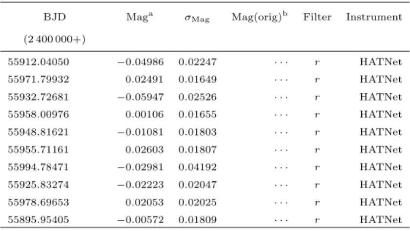
Table 4. Differential Photometry of HAT-P-68

BJD Mag^a σMag Mag(orig)^b Filter Instrument

(2 400 000+)

55912.04050 −0.04986 0.02247 · · · r HATNet

55971.79932 0.02491 0.01649 · · · r HATNet

55932.72681 −0.05947 0.02526 · · · r HATNet

55958.00976 0.00106 0.01655 · · · r HATNet

55948.81621 −0.01081 0.01803 · · · r HATNet

55955.71161 0.02603 0.01807 · · · r HATNet

55994.78471 −0.02981 0.04192 · · · r HATNet

55925.83274 −0.02223 0.02047 · · · r HATNet

55978.69653 0.02053 0.02025 · · · r HATNet

55895.95405 −0.00572 0.01809 · · · r HATNet

a The out-of-transit level has been subtracted. For the HATNet light curve, these magnitudes have been detrended using the EPD and TFA procedures prior to fitting a transit model to the light curve. For the follow-up light curves derived for instruments other than HATNet, these magnitudes have been detrended with the EPD and TFA procedure, carried out simultaneously with the transit fit.

b Raw magnitude values without application of the EPD and TFA procedure.

This is only reported for the follow-up light curves.

Note— This table is available in a machine-readable form in the online journal.

An abdriged version is shown here for guidance regarding its form and content.

The data are also available on the HATNet website athttp://www.hatnet.org.

(9)

system were combined, we place 5σlower limits on the differential magnitude between a putative companion and the primary star as a function of angular separation following the method described in Horch et al.

(2011). These limits are shown in Figure 5. We find ²⁹⁵ limiting magnitude differences at 0.^′′2 of ∆m692 >3.07 and ∆m880>2.68.

In addition to the companion limits based on the WIYN 3.5 m/DSSI observations we also queried the UCAC 4 catalog (Zacharias et al. 2013), and the ³⁰⁰ Gaia DR1 catalog (Gaia Collaboration et al. 2016) for neighbors within 20^′′ that may dilute either the HATNet or KeplerCam photometry. We find no such neighbors. Additionally, the Gaia DR2 catalog (Gaia Collaboration et al. 2018) shows no neighbors ³⁰⁵ within 10^′′of HAT-P-68.

3. ANALYSIS

We analyzed the photometric and spectroscopic observations of HAT-P-68 to determine the parameters of the system using the most up-to-date procedures developed ³¹⁰ for HATNet (Hartman et al. 2019;Bakos et al. 2018) In the following, we briefly summarize our analysis methods to accurately determine the stellar and planetary physical parameters and to rule out various false posi-

tive scenarios. ³¹⁵

3.1. Stellar Host Properties

High-precision stellar atmospheric parameters were measured from the I2-free HIRES template spectrum using SPC, yieldingTeff⋆= 4514±50 K, [Fe/H]=−0.140±

0.080,vsini= 0.0±2.0 km s⁻¹, and logg⋆= 4.67±0.10 ³²⁰ (cgs). The resultingTeff⋆and [Fe/H] measurements were included in the global modelling to determine the physical stellar parameters.

We ultimately tried three methods to ascertain these physical parameters. The first two methods compare the ³²⁵ observable properties to two different stellar evolution models. The last method uses empirical relations to derive stellar mass and radius.

3.1.1. Isochrone-based Parameters

Initially, we attempted to compare the Yonsei-Yale ³³⁰ (Y²;Yi et al. 2001) models to the observed light-curve- based stellar density, and the spectroscopically determined values of Teff⋆ and [Fe/H]. This is the method that was followed, for example, in Bakos et al. (2010), and has been previously applied to the majority of pub- ³³⁵ lished transiting planet discoveries from the HATNet project. Note that this was completed prior to the avail- ability of Gaia DR2. Assuming a circular orbit, the best-fit stellar density is more than 3σ lower than the

6.6 6.7 6.8 6.9 7.0 7.1 7.2

1.36 1.38 1.40 1.42 1.44 1.46 1.48 1.50 1.52 1.54 Gabs [mag]

BP₀-RP₀ [mag]

HAT-P-68 [Fe/H] = -0.06 CMD and SED

■

2.0 5.0

12.0

0.70 0.72

10.5 11.0 11.5 12.0 12.5 13.0 13.5 14.0 14.5 15.0 15.5

B g BP V r G i RP J H Ks W1 W2 W3

Observed Magnitude

-0.6-0.4 -0.20.0 0.20.4 0.60.8 1.01.2

B g BP V r G i RP J H Ks W1 W2 W3

∆ Mag

Figure 6. Top:The absolute Gaia G-band magnitude vs.

the dereddened BP −RP color. This measured value is compared to theoretical isochrones (black lines at Gyr ages in black) and stellar evolution tracks (green lines at solar masses in green) from the PARSEC models interpolated at the spectroscopically determined metallicity of the host. The filled blue circle show the measured reddening- and distance- corrected values fromGaiaDR2, while the blue lines indicate the 1σ and 2σ confidence regions, including the estimated systematic errors in the photometry. Middle: The SED as measured via broadband photometry through the fourteen listed filters. We plot the observed magnitudes without cor- recting for distance or extinction. Overplotted are 200 model SEDs randomly selected from the MCMC posterior distribution produced through the global analysis. Bottom: The residuals from the best-fit model SED.

minimum density from theoretical models – that was ³⁴⁰ achieved within the age of the Galaxy for a K dwarf star with a photosphere temperature of 4500 K. This discrepancy between the measured stellar density and older stellar evolution models, such as the Y² models, has been previously reported for other mid K through ³⁴⁵ early M dwarf stars (eg.Boyajian et al. 2012).

Fortunately,Chen et al.(2014b) improved the PAdova- TRieste Stellar Evolution Code (PARSEC;Bressan et al.

2012) models for very low mass stars (< 0.6M_⊙) over

(10)

a wide range of wavelengths. Randich et al. (2018)

350

also demonstrated that Gaia parallaxes can be combined with ground-based datasets to yield robust stellar ages. As such, we opted to use PARSEC models combined with theGaiaDR2 data, followingHartman et al.

(2019).

355

We performed a tri-linear interpolation within a grid of PARSEC model isochrones using Teff⋆, [Fe/H], and the bulk stellar densityρ⋆as the independent variables.

These three variables in turn are directly varied in the global MCMC analysis (Section3.2), or determined di-

360

rectly from parameters that are varied in this fit. The tri-linear interpolation then yields the M⋆,R⋆ L⋆, and age values to associate with each trial set ofTeff⋆, [Fe/H]

andρ⋆. Through this process we restrict the fit to con- sider only combinations of Teff⋆, [Fe/H] and ρ⋆ that

365

match to a stellar model. For K dwarf stars, such as HAT-P-68, which exhibit little evolution over the age of the Galaxy, this is a rather restrictive constraint. Includ- ing this constraint yields a posteriori estimates for the stellar atmospheric parameters of: Teff⋆= 4508±43 K,

370

[Fe/H]=−0.059±0.036, and logg⋆= 4.615±0.013.

Assuming a circular orbit, the PARSEC isochrone- based method yields a stellar mass and radius of 0.6785^+0.0299₋_0.0079M_⊙and 0.6701^+0.0041₋_0.0032R_⊙, respectively, an age of 11.1^+1.1₋_6.9Gyr, and a reddening-corrected distance

375

of 202.93±0.97 pc. These derived parameters are listed in Table5.

Figure 6 shows the comparison between the broad- band photometric measurements and the PARSEC models mentioned above. The top panel is a color-magnitude

380

diagram (CMD) of the Gaia G magnitude versus the dereddened BP−RP color as a filled blue cicle, along with the 1σand 2σconfidence regions in blue lines. We plot a set of [Fe/H]=0.06 isochrones and stellar evolution tracks using black lines and green lines, respectively.

385

The age of each isochrone is listed in black using Gyr units, while the mass of each evolution track is listed in green using solar mass units. The middle panel com- pares 200 model spectral energy distributions (SEDs) to the observed broadband photometry, the latter of which

390

has not been corrected for distance or extinction. The bottom panel shows the residuals from the best-fit model SED. We find that the observed photometry and parallax is consistent with the models.

3.1.2. Empirically Based Parameters

395

As an alternative approach, we also determined the stellar physical parameters following an empirical method similar to that of Stassun et al. (2017). This method effectively combines the bulk stellar density – measured from the transit light curve – with the stellar

400

radius –measured from the effective temperature, parallax and apparent magnitudes in several band-passes – to determine the stellar mass. In practice this is incor- porated into the global MCMC modelling (Section3.2), and theoretical bolometric corrections are used to pre-

405

dict the absolute magnitude in each band-pass from the effective temperature, radius and metallicity of the star. Assuming a circular orbit, this empirical method yields a stellar mass and radius of 0.614±0.055M_⊙ and 0.6720±0.0075R_⊙, respectively, and a reddening-

410

corrected distance of 203.46±1.00 pc. Note that these parameters are not restricted by the isochrones from PARSEC, which is why the uncertainties are larger compared to the uncertainties on the isochrone-based parameters.

415

3.2. Global Modeling

We determined the parameters of the system by car- rying out a joint modeling of the high-precision RVs (fit using a Keplerian orbit), the HATNet and follow- up light curves (fit using aMandel & Agol 2002 transit

420

model with Gaussian priors for the quadratic limb darkening coefficients taken fromClaret et al. 2012,2013and Claret 2018to place Gaussian prior constraints on their values, assuming a prior uncertainty of 0.2 for each coefficient), the catalog broad-band magnitudes, the stellar

425

parallax from Gaia DR2, and the spectroscopically determined atmospheric parameters of the system. These latter stellar observations were modelled using isochrone and empirical-based methods, as discussed above (Sec- tion3.1). This analysis makes use of a differential evolu-

430

tion Markov Chain Monte Carlo procedure (DEMCMC;

ter Braak 2006) to estimate the posterior parameter distributions, which we use to determine the median parameter values and their 1σuncertainties. We included in the analysis broad-band photometry fromGaia DR2,

435

APASS (Henden et al. 2009), 2MASS (Skrutskie et al.

2006), and WISE (Wright et al. 2010) – G, BP, RP, B, V, g, r, i, J, H, Ks, W1, W2, and W3 bands.

To account for dust extinction we included AV as a free-parameter in the model, assumed theCardelli et al.

440

(1989)RV = 3.1 extinction law, and placed a Gaussian prior onAV based on the predicted extinction from the MWDUST 3D Galactic extinction model (Bovy et al.

2016).

For each of the methods that we adopted to model the

445

stellar parameters, we carried out two fits, one where the orbit is assumed to be circular, and another where the eccentricity parameters are allowed to vary in the fit. In both cases we allow the RV jitter (an extra term added in quadrature to the formal RV uncertain-

450

ties) to vary independently for each of the instruments

(11)

used. We find that when the isochrone-based stellar parameters are used, the free eccentricity model yields an eccentricity consistent with zero (e = 0.013±0.013), resulting in a 95% confidence upper limit on the eccen- ⁴⁵⁵ tricity of e < 0.041. We therefore adopt the following parameters for HAT-P-68b assuming a circular orbit: a mass of 0.724±0.043MJ, a radius of 1.072±0.012RJ, and an equilibrium temperature of 1027.8±8.2 K. The equilibrium temperature was calculated assuming zero ⁴⁶⁰ albedo and full redistribution of heat. We give these parameters, as well as others derived from the joint fit, in Table 6. For comparison, when the empirical method is used, and a circular orbit is assumed, we find a planet mass of 0.711±0.038MJ, planet radius ⁴⁶⁵ of 1.072±0.015RJ, and an equilibrium temperature of 1015.0^+14.9₋_5.7 K.

3.3. Excluding False Positive Scenarios

In order to rule out the possibility that HAT-P-68 is a blended stellar eclipsing binary (EB) system, we ⁴⁷⁰ carried out a direct blend analysis of the data following Hartman et al. (2012), with modifications from Hartman et al.(2019). We find that all blended stellar EB models tested can be ruled out – based on their fit to the photometry, parallax, and light curves – with al- ⁴⁷⁵ most 4σ confidence, and conclude that HAT-P-68 is a transiting planet system, and not a blended stellar EB system.

Note that the blend analysis of HAT-P-68 as an unresolved stellar binary with a planet around one stel- ⁴⁸⁰ lar component provides a slight improvement to the fit compared to assuming no such unresolved stellar companion (∆χ² value of−2.93), but the difference is consistent with the expected improvement from adding an additional parameter to the fit. Based on the high- ⁴⁸⁵ spatial-resolution imaging that we have carried out (Sec- tion2.5), any unresolved companion separated by more than∼0.^′′2, must have ∆m >3.07 at 692 nm compared to the transiting planet host. We conclude our findings assuming that there is no stellar companion. ⁴⁹⁰

4. DISCUSSION

In this paper we have presented the discovery of the HAT-P-68 transiting planet system by the HATNet survey. We have found that everyP = 2.2984 days, HAT- P-68b – with a mass of 0.724±0.043MJ, and radius of ⁴⁹⁵ 1.072±0.012RJ– orbits a star of mass 0.6785^+0.0299₋_0.0079M_⊙, and radius 0.6701^+0.0041₋_0.0032R_⊙. As such, the discovery of this planet contributes to the relatively small sample of low-mass (late K dwarf, and M dwarf stars) stars with

known transiting hot Jupiters. ⁵⁰⁰

We compared the newly discovered planet to the previously discovered planets listed in the NASA Exo-

planet Archive as of 2020 February 21. With a semi- major axis of a=0.02996^+0.00043₋_0.00012AU, this planet joins the small but growing sample of 21 known hot Jupiters ⁵⁰⁵ – with well measured masses – in sub-0.05 AU orbits around low mass stars (< 0.8M_⊙). Here, we follow Dawson & Johnson (2018) and restrict hot Jupiters to planets with masses greater than 0.25MJ.

We find that including HAT-P-68b, there are 10 ⁵¹⁰ planetary systems with transit depths > 2.5%, which may be good targets for transmission spectroscopy.

Of these other worlds, those that have already been studied using transmission spectroscopy include WASP- 80b (Mancini et al. 2014; Kirk et al. 2017), WASP-52b ⁵¹⁵ (Kirk et al. 2016; Louden et al. 2017) and WASP-43b (Chen et al. 2014a; Weaver et al. 2020). While HAT- P-68 is much fainter than these hosts in the optical band-pass, it is only 1 mag fainter than WASP-52 in the

K-band. ⁵²⁰

Finally, we note that HAT-P-68 is at an ecliptic latitude of +3^◦, and is thus outside the field of view of the primary NASA TESSmission. It also was not observed during the K2 mission. The discovery of this planet by HATNet demonstrates that in the era of ⁵²⁵ wide-field space-based transit surveys, interesting planets amenable to detailed characterization remain to be discovered, even from the ground.

Acknowledgements—TBD: Update acknowledgements as needed. HATNet operations have been ⁵³⁰ funded by NASA grants NNG04GN74G as well as NNX13AJ15G. Follow-up of HATNet targets has been partially supported through NSF grant AST-1108686.

B.L. is supported by the NSF Graduate Research Fellow- ship, grant no. DGE 1762114. J.H. acknowledges sup- ⁵³⁵ port from NASA grant NNX14AE87G. G.B., J.H. and W.B. acknowledge partial support from NASA grant NNX17AB61G. We acknowledge partial support from the Kepler Mission under NASA Cooperative Agree- ment NCC2-1390 (D.W.L., PI). Data presented in this ⁵⁴⁰ paper are based on observations obtained at the HAT station at the Submillimeter Array of SAO, and the HAT station at the Fred Lawrence Whipple Observa- tory of SAO. We acknowledge the use of the AAVSO Photometric All-Sky Survey (APASS), funded by the ⁵⁴⁵ Robert Martin Ayers Sciences Fund, and the SIMBAD database, operated at CDS, Strasbourg, France. Data presented herein were obtained at the WIYN Observa- tory from telescope time allocated to NN-EXPLORE through the scientific partnership of the National Aero- ⁵⁵⁰ nautics and Space Administration, the National Science Foundataion, and the Natiaonal Optical Astronomy Observatory. This work was supported by a NASA

(12)

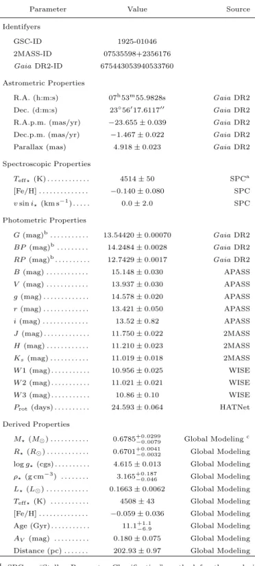
Table 5. Stellar Parameters for HAT-P-68

Parameter Value Source

Identifyers

GSC-ID 1925-01046

2MASS-ID 07535598+2356176

GaiaDR2-ID 675443053940533760 Astrometric Properties

R.A. (h:m:s) 07^h53^m55.9828s GaiaDR2

Dec. (d:m:s) 23^◦56^′17.6117^′′ GaiaDR2

R.A.p.m. (mas/yr) −23.655±0.039 GaiaDR2

Dec.p.m. (mas/yr) −1.467±0.022 GaiaDR2

Parallax (mas) 4.918±0.023 GaiaDR2

Spectroscopic Properties

Teff⋆ (K) . . . . 4514±50 SPC^a [Fe/H] . . . . −0.140±0.080 SPC vsini⋆(km s⁻¹) . . . . . 0.0±2.0 SPC Photometric Properties

G(mag)^b. . . . 13.54420±0.00070 GaiaDR2 BP (mag)^b. . . . 14.2484±0.0028 GaiaDR2 RP(mag)^b. . . . 12.7429±0.0017 GaiaDR2 B(mag) . . . . 15.148±0.030 APASS V (mag) . . . . 13.937±0.030 APASS g(mag) . . . . 14.578±0.020 APASS r(mag) . . . . 13.421±0.050 APASS i(mag) . . . . 13.52±0.82 APASS J(mag) . . . . 11.750±0.022 2MASS H(mag) . . . . 11.210±0.023 2MASS Ks(mag) . . . . 11.019±0.018 2MASS W1 (mag) . . . . 10.956±0.025 WISE W2 (mag) . . . . 11.021±0.021 WISE W3 (mag) . . . . 10.86±0.10 WISE Prot(days) . . . . 24.593±0.064 HATNet Derived Properties

M⋆(M⊙) . . . . 0.6785^+0.0299_−0.0079 Global Modeling^c R_⋆(R⊙) . . . . 0.6701^+0.0041_−0.0032 Global Modeling logg⋆(cgs) . . . . 4.615±0.013 Global Modeling ρ⋆(g cm⁻³) . . . . 3.165^+0.187_−0.046 Global Modeling L⋆(L⊙) . . . . 0.1663±0.0062 Global Modeling Teff⋆ (K) . . . . 4508±43 Global Modeling [Fe/H] . . . . −0.059±0.036 Global Modeling Age (Gyr) . . . . 11.1^+1.1_−6.9 Global Modeling AV (mag) . . . . 0.180±0.075 Global Modeling Distance (pc) . . . . 202.93±0.97 Global Modeling a SPC = “Stellar Parameter Classification” method for the analysis

of high-resolution spectra (Buchhave et al. 2012) applied to the Keck- HIRES I2-free template spectrum of HAT-P-68.

bThe listed uncertainties for theGaiaDR2 photometry are taken from the catalog. For the analysis we assume additional systematic uncertainties of 0.002, 0.005, and 0.003 mag for theG,BP, andRP bands, respectively.

c A posteriori estimates from the Global MCMC analysis of the observations described in Section 3.2. The parameters presented here are derived from an analysis where the stellar parameters are constrained using the PARSEC stellar evolution models (Bressan et al. 2012), and a circular orbit is assumed for the planet.

(13)

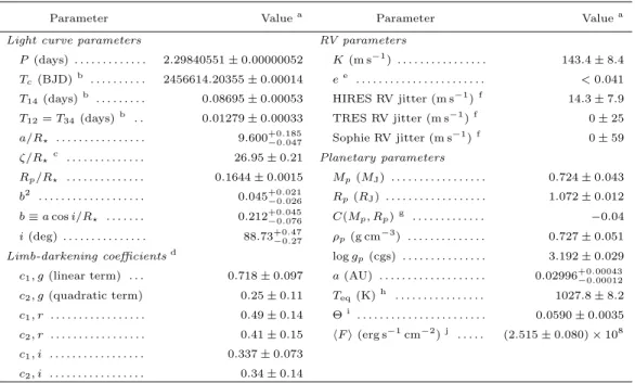
Table 6. Parameters for the planet HAT-P-68b.

Parameter Value^a Parameter Value^a

Light curve parameters RV parameters

P(days) . . . . 2.29840551±0.00000052 K(m s⁻¹) . . . . 143.4±8.4 T_c(BJD)^b . . . . 2456614.20355±0.00014 e^e . . . . <0.041 T14(days)^b . . . . 0.08695±0.00053 HIRES RV jitter (m s⁻¹)^f 14.3±7.9 T12=T34(days)^b . . 0.01279±0.00033 TRES RV jitter (m s⁻¹)^f 0±25 a/R⋆ . . . . 9.600^+0.185_−0.047 Sophie RV jitter (m s⁻¹)^f 0±59 ζ/R_⋆ ^c . . . . 26.95±0.21 Planetary parameters

R_p/R_⋆ . . . . 0.1644±0.0015 M_p(MJ) . . . . 0.724±0.043 b² . . . . 0.045^+0.021_−0.026 Rp(RJ) . . . . 1.072±0.012 b≡acosi/R⋆ . . . . 0.212^+0.045_−0.076 C(Mp, Rp)^g . . . . −0.04 i(deg) . . . . 88.73^+0.47_−0.27 ρp(g cm⁻³) . . . . 0.727±0.051 Limb-darkening coefficients^d loggp(cgs) . . . . 3.192±0.029 c1, g(linear term) . . . 0.718±0.097 a(AU) . . . . 0.02996^+0.00043_−0.00012 c2, g(quadratic term) 0.25±0.11 Teq(K)^h . . . . 1027.8±8.2 c1, r . . . . 0.49±0.14 Θⁱ . . . . 0.0590±0.0035 c2, r . . . . 0.41±0.15 hFi(erg s⁻¹cm⁻²)^j . . . . . (2.515±0.080)×10⁸ c1, i . . . . 0.337±0.073

c2, i . . . . 0.34±0.14

aFor each parameter we give the median value and 68.3% (1σ) confidence intervals from the posterior distribution.

Reported results assume a circular orbit.

b Reported times are in Barycentric Julian Date calculated directly from UTC,withoutcorrection for leap seconds.

Tc: Reference epoch of mid transit that minimizes the correlation with the orbital period. T14: total transit duration, time between first to last contact;T12=T34: ingress/egress time, time between first and second, or third and fourth contact.

c Reciprocal of the half duration of the transit used as a jump parameter in our DE-MC analysis in place ofa/R⋆. It is related toa/R⋆by the expressionζ/R⋆=a/R⋆(2π(1 +esinω))/(P√

1−b²√

1−e²) (Bakos et al. 2010).

dValues for a quadratic law, adopted from the tabulations byClaret(2004) according to the spectroscopic (SPC) parameters listed in Table5.

e The 95% confidence upper-limit on the eccentricity. All other parameters listed are determined assuming a circular orbit for this planet.

f Error term, either astrophysical or instrumental in origin, added in quadrature to the formal RV errors. This term is varied in the fit independently for each instrument assuming a prior that is inversely proportional to the jitter.

gCorrelation coefficient between the planetary massM_pand radiusR_pdetermined from the parameter posterior distribution viaC(M_p, R_p) =h(M_p− hM_pi)(R_p− hR_pi)i/(σ_Mpσ_Rp)i, whereh·iis the expectation value, and σ_xis the std. dev. ofx.

hPlanet equilibrium temperature averaged over the orbit, calculated assuming a Bond albedo of zero, and that flux is reradiated from the full planet surface.

i The Safronov number is given by Θ =¹₂(Vesc/Vorb)²= (a/Rp)(Mp/M⋆) (seeHansen & Barman 2007).

j Incoming flux per unit surface area, averaged over the orbit.