Exploring self-intersected 𝑁 -periodics in the elliptic billiard
Ronaldo Garcia
a∗, Dan Reznik
baFed. Univ. of Goiás, Goiânia, Brazil ragarcia@ufg.br
bData Science Consulting, Rio de Janeiro, Brazil dreznik@gmail.com
Submitted: April 5, 2021 Accepted: February 11, 2022 Published online: February 22, 2022
Abstract
This is a continuation of our simulation-based investigation of𝑁-periodic trajectories in the elliptic billiard. With a special focus on self-intersected trajectories we (i) describe new properties of𝑁= 4family, (ii) derive expres- sions for quantities recently shown to be conserved, and to support further experimentation, we (iii) derive explicit expressions for vertices and caustic semi-axes for several families. Finally, (iv) we include links to several anima- tions of the phenomena.
Keywords:Invariant, elliptic, billiard, turning number, self-intersected AMS Subject Classification:51M04, 51N20, 51N35, 68T20
1. Introduction
This is a continuation of our simulation-based investigation of periodic trajectories in the elliptic billiard, i.e., Poncelet families of polygons interscribed between two confocal conics (see Appendix A for a review).
Here we focus on trajectories which are self-intersected, i.e., which wrap around the inner conic, or caustic, more than once (i.e., their turning number is greater
∗Supported by PRONEX/CNPq/FAPEG 2017-10-26-7000-508.
Accepted manuscript
doi: https://doi.org/10.33039/ami.2022.02.001 url: https://ami.uni-eszterhazy.hu
1
than one [24]). Figure 1 (resp. 2) illustrate cases where the caustic is an ellipse (resp. hyperbola).
Figure 1. A simple (left), and two self-intersecting (middle, right) 7-periodics in the elliptic billiard. In the article the latter two are labeled “type I”, and “type II” (turning number 2 and, 3 respec-
tively). Video 1: youtu.be/yzBG8rgPUP4 Video 2: youtu.be/BRQ39O9ogNE
Specifically, we (i) describe some curious Euclidean properties, loci, and invari- ants of the𝑁 = 4self-intersected family (Section 3); (ii) derive expressions for some conserved quantities presented in [20, 21], for both simple and self-intersected cases (Section 4). Interestingly, we identify a few situations where quantities conserved elsewhere become variable (reasons are unclear).
One of our goals is to encourage and support further simulation work. Toward that end, we include links to animated phenomena in the caption of most figures, all of which appear on Table 2. In Appendix B we provide expressions for both vertices and caustics for several families. Appendix C lists most symbols used herein.
1.1. Related work
Birkhoff provides a method to compute the number of possible Poncelet𝑁-perio- dics, simple or not [7]. For example, for 𝑁 = 5,6,7,8 there are 1,2,2,3 distinct self-intersected closed trajectories, respectively. In [18] expressions are derived for caustic parameters which produce various types of 𝑁-periodics in the elliptic bil- liard. Points of self-intersections of Poncelet 𝑁-periodics are located on confocal conics of the associated Poncelet grid [16, 22, 25]. A kinematic analysis of the geom- etry of𝑁=periodics using Jacobian elliptic functions is proposed in [24]. Works [13, 19] derive explicit expressions for some invariants in the𝑁= 3case (billiard trian- gles). Additional constructions derived from N-periodics (e.g., pedals, antipedals, etc.) are considered in [20], augmenting the list of elliptic billiard invariants to 80.
In recent publications [13, 19, 21] we have described several Euclidean quantities which remain invariant over a given family, some of which have been subsequently proved [2, 5, 8].
2. Preliminaries
Throughout this article we assume the elliptic billiard is the ellipse:
𝑓(𝑥, 𝑦) =(︁𝑥 𝑎
)︁2
+(︁𝑦 𝑏
)︁2
= 1, 𝑎 > 𝑏 >0.
Below we refer to trajectories with turning number 1, 2, 3, and 4, by simple, type I, type II, and type III, respectively.
2.1. A word about our proof method
We omit most proofs as they have been produced by a consistent process, namely:
(i) using the expressions in Appendix B, find the vertices an axis-symmetric 𝑁- periodic, i.e., whose first vertex𝑃1= (𝑎,0); (ii) obtain a symbolic expression for the invariant of interest; (iii) derive an expression for the given quantity for a generic trajectory parametrized by 𝑡; (iv) using CAS simplification, show that 𝑡 can be eliminated, i.e., that (iii) reduces to (ii).
3. Properties of self-intersected 4-periodics
The family of simple 4-periodics in the elliptic billiard are parallelograms [9]. In this section consider self-intersected 4-periodics whose caustic is a confocal hyperbola;
see Figure 2. We start deriving simple facts about them and then proceed to certain elegant properties.
Proposition 3.1. The perimeter𝐿 of the self-intersected 4-periodic is given by:
𝐿= 4𝑎2
𝑐 , with 𝑐2=𝑎2−𝑏2. (3.1)
Proof. Since perimeter is constant, use as the 𝑁 = 4 candidate the centrally- symmetric one, Figure 2 (right). Its upper-right vertex 𝑃1 = (𝑥1, 𝑦1) is such that it reflects a vertical ray toward−𝑃1, and this yields:
𝑃1= (𝑥1, 𝑦1) = [︃𝑎√
𝑎2−2𝑏2 𝑏𝑐 ,𝑏
𝑐 ]︃
.
Since 𝑃2 =−𝑃1 its perimeter is𝐿= 2(|2𝑃1|+ 2𝑦1) and this can be simplified to (3.1), invariant over the family.
with𝑎/𝑏≥√
2. At𝑎/𝑏=√
2the family is a straight line from top to bottom vertex of the elliptic billiard, Figure 2 (left).
Observation 3.2. At𝑎/𝑏=√︀
1 +√
2≃1.55377the two self-intersecting segments of the bowtie do so at right-angles.
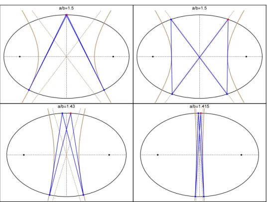
Figure 2. In the top left (resp. top right) an𝑁= 4self-intersected trajectory is shown near its “doubled up” (resp. almost symmetric) position. In both cases trajectory segments are tangent to a hy- perbolic caustic (brown). As the aspect ratio of the elliptic billiard decreases (bottom left and right), the family is squeezed into an ever narrower space between the approaching branches of the caus-
tic. Video: youtu.be/cCYxN7ueGV4
Observation 3.3. At𝑎/𝑏≃1.55529 the perimeter of the bowtie equal that of the elliptic billiard.
Referring to Figure 3:
Proposition 3.4. The𝑁 = 4self-intersected family has zero signed orbit area and zero sum of signed cosines, i.e., both are invariant. The same two facts are true for its outer polygon. Furthermore the latter has zero sum of double-angle signed cosines.
Proof. This stems from the fact all self-intersected 4-periodics are symmetric with respect to the elliptic billiard’s minor axis.
Referring to Figure 3, as in Appendix B.2, let vertex𝑃1of the self-intersected 4- periodic be parametrized as𝑃1(𝑢) =[︀
𝑎𝑢, 𝑏√
1−𝑢2]︀, with|𝑢|≤𝑐𝑎2
√𝑎2−2𝑏2. Then:
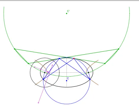
Figure 3. The vertices of the self-intersected 4-periodic (blue) are concyclic with the foci of the elliptic billiard on a circle (dashed blue) centered on 𝐶. The inversive polygon (pink segment) with respect to a unit circle𝐶† (dashed black) centered on the left focus degenerates to a segment along the radical axis of the two circles.
The vertices of the outer polygon (green) are also concyclic with the foci on a distinct circle (dashed green) centered on 𝐶′. Therefore the outer’s inversive polygon (dotted pink) is also a segment along the radical axis of this circle with𝐶†. Note the two radical axes are
dynamically perpendicular.
Video 1: youtu.be/207Ta31Pl9I Video 2: youtu.be/4g-JBshX10U
Theorem 3.5. The four vertices of the self-intersected 4-periodic (resp. outer poly- gon) are concyclic with the two foci of the elliptic billiard, on a circle𝒞 of variable radius𝑅 (resp.𝑅′) whose center𝐶 (resp.𝐶′) lies on the y axis. These are given by:
𝐶= [︂
0,𝑐2𝑢2−𝑎2+ 2𝑏2 2𝑏√
1−𝑢2 ]︂
, 𝐶′=
[︃
0,− 2𝑏𝑐2√ 1−𝑢2 𝑎2+ (𝑢2−2)𝑐2
]︃
, 𝑅=𝑎2−𝑐2𝑢2
2𝑏√
1−𝑢2, 𝑅′= 𝑐(𝑐2𝑢2−𝑎2) 𝑎2+ (𝑢2−2)𝑐2·
Corollary 3.6. The half harmonic mean of 𝑅2 and 𝑅′2 is invariant and equal to 𝑐2=𝑎2−𝑏2, i.e., 1/𝑅2+ 1/𝑅′2= 1/𝑐2.
Note: the above Pythagorean relation implies that the polygon whose vertices are a focus, and the inversion of𝐶, 𝐶′, 𝑂(center of the elliptic billiard) with respect to a unit circle centered on said focus, is a rectangle of sides 1/𝑅 and 1/𝑅′ and diagonal1/𝑐.
Remarkably:
Corollary 3.7. Over the self-intersected 𝑁 = 4 family, the power of the origin with respect to both𝒞 and𝒞′ is invariant and equal to𝑏2−𝑎2.
Referring to Figure 4,𝑁 = 4self-intersected trajectories areanti-parallelograms [27]: these are images of vertices of a parallelogram reflected on opposite diagonals.
A well-know property is that the midpoints of its four segments are collinear on a horizontal line parallel to a diagonal.
Observation 3.8. The locus of midpoints of 𝑁 = 4 self-intersected segments is an ∞-shaped quartic curve given by:
𝑐2(𝑏2𝑥2+𝑎2𝑦2)2−𝑏4𝑎2(︀
(𝑎2−2𝑏2)𝑥2−𝑎2𝑦2)︀
= 0.
Furthermore, the above quartic is tangent to the confocal hyperbolic caustic at its vertices[±𝑎√
𝑎2−2𝑏2/𝑐,0].
Figure 4. The midpoints of each of the four segments of self- intersected 4-periodics are collinear on a horizontal line. Their locus is an ∞-shaped quartic which touches the caustic at its vertices.
Video: youtu.be/GZCrek7RTpQ
Let𝒫† (resp. 𝒬†) denote the inversive polygon of 4-periodics (resp. its outer polygon) wrt a unit circle𝒞† centered on one focus. From properties of inversion:
Corollary 3.9. 𝒫† (resp.𝒬†) has four collinear vertices, i.e., it degenerates to a segment along the radical axis of𝒞† and𝒞 (resp.𝒞′).
Proposition 3.10. The two said radical axes are perpendicular.
Proof. It is enough to check that the vectors 𝐶−[−𝑐,0]and 𝐶′−[−𝑐,0] are or- thogonal. Observe that when𝑢2= (𝑎2−2𝑏2)/𝑐= (2𝑐2−𝑎2)/𝑐 the outer polygon is contained in the horizontal axis.
Observation 3.11. The pairs of opposite sides of the outer polygon to self-intersec- ted 4-periodics intersect at the top and bottom of the circle (𝐶, 𝑅) on which the 4-periodic vertices are concyclic.
4. Deriving both simple and self-intersected invari- ants
In this section, we derive expressions for selected invariants introduced in [20], specifically for “low-N” cases, e.g.,𝑁 = 3,4,5,6,8. In that publication, each invari- ant is identified by a 3-digit code, e.g.,𝑘101,𝑘102, etc. Table 1 lists the invariants considered herein. The quantities involved are defined next.
Table 1. List of selected invariants taken from [20] as well as the low-𝑁 cases (column “derived”) for expressions are derived herein, where 𝑁 refers to simple 𝑁-periodics, and 𝑁𝑖 (resp. 𝑁𝑖𝑖) refers to type I (resp. type II) 𝑁-periodics. Refer to Table 3 for the meaning of symbols in column “invariant”. † 𝐿1 was co-discovered with P. Roitman. A closed-form expression for𝑘119was derived by
H. Stachel; see (A.1).
code invariant valid N derived proofs
𝑘101 ∑︀cos𝜃𝑖 all 𝐽𝐿−𝑁 [2, 5]
𝑘102 ∏︀
cos𝜃′𝑖 all 3,4,5,5𝑖,6,6𝑖,6𝑖𝑖 [2, 5]
𝑘103 𝐴′/𝐴 odd 3,5,5𝑖 [2, 8]
𝑘104 ∑︀
cos(2𝜃𝑖′) all 3,4,4𝑖,5,5𝑖,6,6𝑖,8 [1]
𝑘105 ∏︀sin(𝜃𝑖/2) odd 3,5,5𝑖 [1]
𝑘106 𝐴′𝐴 even 4,4𝑖,6,6𝑖,6𝑖𝑖 [8]
𝑘110 𝐴 𝐴′′ even 4,4𝑖,6,6𝑖,6𝑖𝑖 ?
†𝑘119 ∑︀
𝜅2/3𝑖 all 3,4,6 [2, 23]
𝑘802,𝑎 ∑︀
1/𝑑1,𝑖 all 3,4,6 [2]
𝑘803 𝐿†1 all 3,4,6 ?
†𝑘804 ∑︀
cos𝜃†1,𝑖 ̸=4 3 ?
𝑘805,𝑎 𝐴 𝐴†1 ≡0 (mod 4) 4,4𝑖,8 ?
𝑘806 𝐴/𝐴†1 ≡2 (mod 4) 6 ?
𝑘807 𝐴†1.𝐴†2 odd 3 ?
Let𝜃𝑖 denote the ith N-periodic angle. Let𝐴the signed area of an N-periodic.
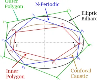
Referring to Figure 5, singly-primed quantities (e.g.,𝜃′𝑖,𝐴′, etc.), etc., always refer to theouter polygon: its sides are tangent to the elliptic billiard at the𝑃𝑖. Likewise, doubly-primed quantities (𝜃′′𝑖,𝐴′′, etc.) refer to theinner polygon: its vertices lie at the touchpoints of N-periodic sides with the caustic. More details on said quantities appear in Appendix A.
Recall𝑘101=𝐽𝐿−𝑁, as introduced in [5, 19].
Referring to Figure 6, the𝑓1-inversive polygonhas vertices at inversions of the 𝑃𝑖 with respect to a unit circle centered on 𝑓1. Quantities such as 𝐿†1, 𝐴†1, etc., refer to perimeter, area, etc. of said polygon.
Figure 5. The 𝑁-periodic (blue), is associated with an outer (green) and an inner (red) polygons. The former’s sides are tan- gent to the billiard (black) at each 𝑁-periodic vertex; the latter’s vertices are the tangency points of𝑁-periodics sides to the confocal
caustic (brown). Video: youtu.be/PRkhrUNTXd8
Figure 6. Focus-inversive 5-periodic (pink) whose vertices are in- versions of the𝑃𝑖(blue) with respect to a unit circle (dashed black) centered on𝑓1. It turns out its perimeter is also invariant over the
family as is the sum of its spoke lengths (pink lines) Video: youtu.be/wkstGKq5jOo.
4.1. Invariants for 𝑁 = 3
As before, let 𝛿 = √
𝑎4−𝑎2𝑏2+𝑏4. For𝑁 = 3 explicit expressions for 𝐽 and 𝐿 have been derived [13]:
𝐽 =
√2𝛿−𝑎2−𝑏2
𝑐2 , 𝐿= 2(𝛿+𝑎2+𝑏2)𝐽. (4.1)
When𝑎=𝑏,𝐽 =√
3/2 and when𝑎/𝑏→ ∞,𝐽 →0.
Proposition 4.1. For𝑁 = 3,𝑘102= (𝐽𝐿)/4−1. Proof. We’ve shown ∑︀3
𝑖=1cos𝜃𝑖 =𝐽𝐿−3 is invariant for the 𝑁 = 3 family [13].
For any triangle ∑︀3
𝑖=1cos𝜃𝑖 = 1 +𝑟/𝑅 [28], so it follows that 𝑟/𝑅 = 𝐽𝐿−4 is also invariant. Let 𝑟ℎ, 𝑅ℎ be the Orthic Triangle’s Inradius and Circumradius.
The relation 𝑟ℎ/𝑅ℎ = 4∏︀3
𝑖=1|cos𝜃𝑖| is well-known [28, Orthic Triangle]. Since a triangle is the Orthic of its Excentral Triangle, we can write 𝑟/𝑅= 4∏︀3
𝑖=1cos𝜃𝑖′, where 𝜃′𝑖 are the Excentral angles which are always acute [28] (absolute value can be dropped), yielding the claim.
Proposition 4.2. For𝑁 = 3,𝑘103=𝑘109= 2/(𝑘101−1) = 2/(𝐽𝐿−4).
Proof. Given a triangle 𝐴′ (resp. 𝐴′′) refers to the area of the Excentral (resp.
Extouch) triangles. The ratios 𝐴′/𝐴 and 𝐴/𝐴′′ are equal. Actually, 𝐴′/𝐴 = 𝐴/𝐴′′ = (𝑠1𝑠2𝑠3)/(𝑟2𝐿), where 𝑠𝑖 are the sides, 𝐿 the perimeter, and 𝑟 the In- radius [28, Excentral, Extouch]. Also known is that 𝐴′/𝐴 = 2𝑅/𝑟 [14]. Since 𝑟/𝑅=∑︀3
𝑖=1cos𝜃𝑖−1 =𝑘101−1[28, Inradius], the result follows.
Proposition 4.3. For𝑁 = 3,𝑘104=−𝑘101 and is given by:
𝑘104=
(︀𝑎2+𝑏2)︀ (︀
𝑎2+𝑏2−2𝛿)︀
𝑐4 = 3−𝐽𝐿.
Proposition 4.4. For𝑁 = 3,𝑘105= (𝐽𝐿)/4−1 =𝑘102.
Proof. Let 𝑟, 𝑅 be a triangle’s Inradius and Circumradius. The identity 𝑟/𝑅 = 4∏︀3
𝑖=1sin(𝜃𝑖/2) holds for any triangle [28, Inradius], which with Proposition 4.1 This completes the proof.
Proposition 4.5. For𝑁 = 3,𝑘119 is given by:
(𝑘119)3= 2𝐽3𝐿
(𝐽𝐿−4)2, 𝑘119= 𝑎2+𝑏2+𝛿 (𝑎𝑏)43 . Proof. Use the expressions for𝐿, 𝐽 in (4.1).
Proposition 4.6. For𝑁 = 3:
𝑘802,𝑎= 𝑎2+𝑏2+𝛿 𝑎𝑏2 = 𝐽√
2√︀
𝐽𝐿+√
9−2𝐽𝐿−3
𝐽𝐿−4 ,
𝑘803=𝜌
√︀(8𝑎4+ 4𝑎2𝑏2+ 2𝑏4)𝛿+ 8𝑎6+ 3𝑎2𝑏4+ 2𝑏6
𝑎2𝑏2 ,
𝑘804= 𝛿(𝑎2+𝑐2−𝛿) 𝑎2𝑐2 , 𝑘807= 𝜌8
8𝑎8𝑏2
[︀(︀𝑎4+ 2𝑎2𝑏2+ 4𝑏4)︀
𝛿+𝑎6+ (3/2)𝑎4𝑏2+ 4𝑏6]︀
.
Note: 𝜌 is the radius of the inversion circle, included above for unit consistency.
By default𝜌= 1.
4.2. Invariants for 𝑁 = 4
Proposition 4.7. For simple 𝑁 = 4,𝑘102= 0.
Proof. Simple 4-periodics are parallelograms [9] whose outer polygon is a rectangle inscribed in Monge’s Orthoptic Circle [19]. This finishes the proof.
Proposition 4.8. For simple 𝑁 = 4,𝑘104=−4.
Proof. As in Proposition 4.7, outer polygon is a rectangle.
Let𝜅𝑎= (𝑎𝑏)−2/3 denote the affine curvature of the ellipse and𝑟𝑚=√ 𝑎2+𝑏2 the radius of Monge’s orthoptic circle [28].
Proposition 4.9. For simple 𝑁 = 4:
𝑘106= 8𝑎2𝑏2, 𝑘110= 2𝑎4𝑏4 (𝑎2+𝑏2)2, 𝑘119= 2(𝑎2+𝑏2)
(𝑎𝑏)43 = 2(𝜅𝑎𝑟𝑚)2, 𝑘802,𝑎=2(𝑎2+𝑏2) 𝑎𝑏2 , 𝑘803= 4𝜌2√
𝑎2+𝑏2
𝑏2 , 𝑘805,𝑎= 4.
Note: when𝑏= 1,𝑘803 is equal to the perimeter of the 4-periodic; see (B.1).
Counter-example 4.10. Experimentally,𝑘804is invariant for all simple N-perio- dics, except when𝑁 = 4.
Restating results from Proposition 3.4:
Observation 4.11. Over self-intersected𝑁= 4,𝑘101=𝑘104= 0. Since𝐴is null, so are 𝑘106,𝑘110, and𝑘805,𝑎.
We leave as exercises the derivation of expressions for 𝑘102, 𝑘119, 𝑘802,𝑎, and 𝑘803 over self-intersected𝑁 = 4.
4.3. Invariants for 𝑁 = 5
As seen in Appendix B, the vertices of 5-periodics can only be obtained via an implicitly-defined caustic. Namely, we first numerically obtain the caustic semi-axes and then compute a axis-symmetric polygon tangent to it. Note that both simple and self-intersected 5-periodics possess an elliptic confocal caustic; see Figure 7.
Proposition 4.12. For simple (resp. self-intersected)𝑁 = 5,𝑘102 is given by the largest negative (resp. positive) real root of the following 6th-degree polynomial:
𝑘102: 1024𝑐20𝑥6+ 2048(𝑎4+𝑎3𝑏−𝑎𝑏3+𝑏4)(𝑎4−𝑎3𝑏+𝑎𝑏3+𝑏4)𝑐12𝑥5 + 256(4𝑎12−𝑎10𝑏2+ 32𝑎8𝑏4−22𝑎6𝑏6+ 32𝑎4𝑏8−𝑎2𝑏10+ 4𝑏12)𝑐8𝑥4
−64𝑎2𝑏2(4𝑎12−27𝑎10𝑏2+ 38𝑎8𝑏4−126𝑎6𝑏6+ 38𝑎4𝑏8−27𝑎2𝑏10+ 4𝑏12)𝑐4𝑥3
−16𝑎6𝑏6(7𝑎8−96𝑎6𝑏2+ 114𝑎4𝑏4−96𝑎2𝑏6+ 7𝑏8)𝑥2
−8𝑎8𝑏8(7𝑎4+ 30𝑎2𝑏2+ 7𝑏4)𝑥−𝑎10𝑏10= 0.
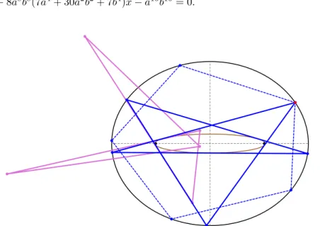
Figure 7. A simple (blue) and self-intersected (dashed blue) 5- periodic, as well as the former’s focus-inversive polygon (pink).
Video: youtu.be/LuLtbwkfSbc
Proposition 4.13. For simple (resp. self-intersected)𝑁 = 5,𝑘103 is given by the smallest (resp. largest) real root greater than 1 of the following 6th-degree polyno- mial:
𝑘103:𝑎6𝑏6𝑥6−2𝑏2𝑎2(︀
4𝑎8−𝑎6𝑏2−𝑎2𝑏6+ 4𝑏8)︀
𝑥5
−𝑏2𝑎2(︀
4𝑎8+ 19𝑎6𝑏2−62𝑎4𝑏4+ 19𝑎2𝑏6+ 4𝑏8)︀
𝑥4 + 12𝑏2𝑎2(︀
𝑎4+𝑏4)︀
𝑐4𝑥3+(︀
4𝑎8+ 19𝑎6𝑏2+ 66𝑎4𝑏4+ 19𝑎2𝑏6+ 4𝑏8)︀
𝑐4𝑥2 +(︀
2𝑎8+ 12𝑎6𝑏2+ 36𝑎4𝑏4+ 12𝑎2𝑏6+ 2𝑏8)︀
𝑐4𝑥−𝑐12.
Proposition 4.14. For simple (resp. self-intersected)𝑁 = 5,𝑘104 is given by the only negative (resp. smallest largest) real root of the following 6th-degree polynomial:
𝑐12𝑥6−2(𝑎4+ 10𝑎2𝑏2+𝑏4)𝑐8𝑥5−(37𝑎4−6𝑎2𝑏2+ 37𝑏4)𝑐8𝑥4 + 4(5𝑎8+ 92𝑎6𝑏2+ 62𝑎4𝑏4+ 92𝑎2𝑏6+ 5𝑏8)𝑐4𝑥3
+ (423𝑎12−354𝑎10𝑏2+ 2713𝑎8𝑏4−4796𝑎6𝑏6+ 2713𝑎4𝑏8−354𝑎2𝑏10+ 423𝑏12)𝑥2 + (270𝑎12+ 740𝑎10𝑏2−3630𝑎8𝑏4+ 7160𝑎6𝑏6−3630𝑎4𝑏8+ 740𝑎2𝑏10+ 270𝑏12)𝑥
−675𝑎12−850𝑎10𝑏2+ 1075𝑎8𝑏4−3900𝑎6𝑏6+ 1075𝑎4𝑏8−850𝑎2𝑏10−675𝑏12.
Proposition 4.15. For simple (resp. self-intersected)𝑁 = 5,𝑘105 is given by the largest positive real root (resp. the symmetric value of the largest negative root) of the following 6th-degree polynomial:
210𝑐20𝑥6+ 210(2𝑎12+𝑎10𝑏2+ 26𝑎8𝑏4+ 70𝑎6𝑏6+ 26𝑎4𝑏8+𝑎2𝑏10+ 2𝑏12)𝑐8𝑥5 + 28(4𝑎12+ 30𝑎10𝑏2+ 71𝑎8𝑏4+ 350𝑎6𝑏6+ 71𝑎4𝑏8+ 30𝑎2𝑏10+ 4𝑏12)𝑐8𝑥4 + 26𝑎2𝑏2(4𝑎12+ 9𝑎10𝑏2−318𝑎8𝑏4−126𝑎6𝑏6−318𝑎4𝑏8+ 9𝑎2𝑏10+ 4𝑏12)𝑐4𝑥3
−26𝑎2𝑏2(8𝑎16−53𝑎14𝑏2+ 253𝑎12𝑏4−1041𝑎10𝑏6+ 1650𝑎8𝑏8
−1041𝑎6𝑏10+ 253𝑎4𝑏12−53𝑎2𝑏14+ 8𝑏16)𝑥2
−24𝑎2𝑏2(16𝑎16−12𝑎14𝑏2+ 5𝑎12𝑏4+𝑎10𝑏6+ 2𝑎8𝑏8+𝑎6𝑏10 + 5𝑎4𝑏12−12𝑎2𝑏14+ 16𝑏16)𝑥
−𝑎10𝑏10.
4.4. Invariants for 𝑁 = 6
Referring to Figure 5 (right):
Proposition 4.16. For simple 𝑁= 6:
𝑘102=𝑎2𝑏2/(4(𝑎+𝑏)4) = (𝐽𝐿−4)2/64, 𝑘104=𝑘101=𝐽𝐿−6,
𝑘106=4𝑏2(2𝑎+𝑏)𝑎2(𝑎+ 2𝑏)
(𝑎+𝑏)2 =−(𝐽𝐿−12) (𝐽𝐿−4)2
16𝐽4 ,
𝑘110=4𝑎3𝑏3(2𝑎+𝑏)2(𝑎+ 2𝑏)2
(𝑎+𝑏)6 =−(𝐽𝐿−12)2(𝐽𝐿−4)3 256𝐽4 , 𝑘3119= 25𝐽5𝐿3
(𝐽𝐿−4)4, 𝑘802,𝑎=2(𝑎2+𝑎𝑏+𝑏2)
𝑎𝑏2 = 4𝐽2𝐿(︀
1 +√
𝐽𝐿−3)︀
(𝐽𝐿−4)2 , 𝑘803= 2𝜌2(2𝑎2+ 2𝑎𝑏−𝑏2)/(𝑎𝑏2),
𝑘806= 4𝜌−4𝑎3𝑏4/((2𝑎−𝑏)(𝑎+𝑏)2).
4.5. 𝑁 = 6 self-intersecting
Only two 𝑁 = 6 topologies can produce closed trajectories, both with two self- intersections. These will be referred to as type I and type II, and are depicted in Figures 8, and 9, respectively.
Proposition 4.17. For𝑁 = 6type I:
𝑘102=𝑎2𝑏2/(4(𝑎−𝑏)4) = (𝐽 𝐿−4)2/64,
𝑘104=−2(𝑎2−4𝑎𝑏+𝑏2)
(𝑎−𝑏)2 =𝐽𝐿−6 =𝑘101,
𝑘106= 4𝑎2𝑏2(𝑎−2𝑏)(2𝑎−𝑏)/(𝑎−𝑏)2=−(𝐽𝐿−12)(𝐽𝐿−4)2/(16𝐽4), 𝑘110=−4𝑎3𝑏3(𝑎−2𝑏)2(2𝑎−𝑏)2
(𝑎−𝑏)6 = (𝐽𝐿−12)2(𝐽𝐿−4)3 28𝐽4 .
Figure 8. Type I self-intersected 6-periodic (blue) and its doubled- up configuration (dashed red), both tangent to a hyperbolic confocal caustic (brown). Its asymptotes (dashed black) pass through the center of the elliptic billiard. Also shown are the outer (green) and
inner (dark red) polygons. Video: youtu.be/fOD85MNrmdQ
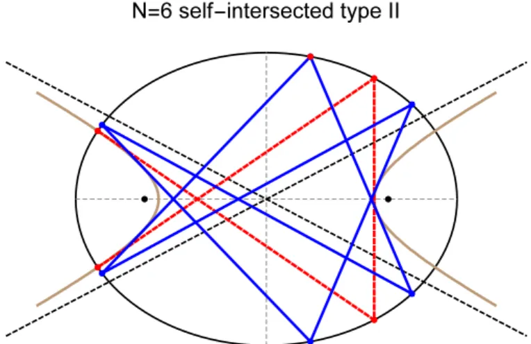
Figure 9. Self-intersected 6-periodic (type II) shown both at one of its doubled-up configurations (dashed red) and in general posi- tion (blue). Segments are tangnet to a hyperbolic confocal caustic (brown) whose asymptotes (dashed black) pass through the cen- ter of the elliptic billiard. Also shown is the outer polygon (green) which in this case is always simple. Video:youtu.be/gQ-FbSq7wWY
Proposition 4.18. For𝑁 = 6type II:
𝑘102=𝑎2(𝑎−𝑐)2/(4𝑐4) = (𝐽𝐿−8)2(𝐽𝐿−4)2/1024, 𝑘104=2(𝑎2−𝑎𝑐+𝑐2)(𝑎2−𝑎𝑐−𝑐2)
𝑐4 = (𝐽2𝐿2−12𝐽𝐿+ 16)(𝐽2𝐿2−12𝐽𝐿+ 48)
128 ,
𝑘106=𝑘110= 0.
Note (i) in contrast with the above, 𝑘104 =𝑘101=𝐽𝐿−6for both𝑁 = 6simple and type I, and (ii) 𝑘106 and𝑘110are nil since both𝐴and𝐴′ vanish.
Counter-example 4.19. Experimentally,𝑘804is invariant for𝑁= 6simple, and type I. However, it is variable for 𝑁 = 6type II.
4.6. Invariants for 𝑁 = 8
Referring to Figure 10:
Figure 10. The outer polygon (green) to a simple 8-periodic has null sum of double cosines. Video: youtu.be/GEmV_U4eRIE
Proposition 4.20. For simple𝑁 = 8,𝑘102is given by(1/212)(𝐽𝐿−4)2(𝐽𝐿−12)2. Proposition 4.21. For𝑁 = 8,𝑘104= 0.
Proof. Using the CAS, we checked that𝑘104vanishes for an 8-periodic in the “hor- izontal” position, i.e., 𝑃1 = (𝑎,0). Since 𝑘104 is invariant [2], this completes the proof.
4.7. 𝑁 = 8 self-intersected
There are 3 types of self-intersected 8-periodics [6], here called type I, II, and III.
These correspond to trajectories with turning numbers of 0, 2, and 3, respectively.
These are depicted in Figures 11, 12, and 13.
Observation 4.22. The signed area of 𝑁 = 8type I is zero.
Referring to Figure 13, the following is related to the Poncelet Grid [16] and the Hexagramma Mysticum [3]:
Observation 4.23. The outer polygon to𝑁 = 8type III is inscribed in an ellipse.
Figure 11. Self-intersecting 8-periodic of type I (blue) and its doubled-up configuration (dashed red) in 𝑎/𝑏= 3 ellipse. Trajec- tory segments are tangent to a confocal hyperbolic caustic (brown).
Video: youtu.be/5Lt9atsZhRs
Figure 12. Four positions of a type-II self-intersecting 8-periodic trajectory (blue) in an 𝑎/𝑏 = 1.2 elliptic billiard, at four differ- ent locations of a starting vertex (red). In general position, these have turning number 2. Also shown is confocal hyperbolic caustic
(brown). Video: youtu.be/JwD_w5ecPYs
Figure 13. A type-III self-intersected 8-periodic trajectory (blue) and its doubled-up configuration (dashed red) in an𝑎/𝑏 = 1.1el- liptic billiard (shown rotated by 90∘ to save space). The turning number is 3. The confocal caustic is an ellipse (brown). Also shown is the outer polygon (green) whose vertices are inscribed in an axis- aligned, concentric ellipse (dashed green), a result related to [3].
Video: youtu.be/93xpGnDxyi0
5. When invariants are variable
The sum of focus-inversive cosines (𝑘804) is invariant in all N-periodics so far stud- ied, excepting 𝑁 = 4 simple and𝑁 = 6 type II; see Counter-examples 4.10 and 4.19. Notice that for the former the area of simple 4-periodics is non-zero while the sum of cosines vanishes; in the latter case the situation reverses: the area of type II 6-periodics vanishes and the sum of cosines is non-zero. Could either vanishing quantity be the reason 𝑘804 becomes variable, e.g., is this introducing a pole in the meromorphic functions on the elliptic curve assumed in the proof of invariants in [2]?
6. Videos
Animations illustrating some of the above phenomena are listed on Table 2.
Acknowledgments
The authors are grateful for the constructive comments by the referee. We would also like to thank Arseniy Akopyan, Jair Koiller, Pedro Roitman, Richard Schwartz,
Table 2. Videos illustrating some phenomena. The last column is clickable and/or provides the YouTube code.
id Title youtu.be/<...>
01 𝑁= 3−6orbits and caustics Y3q35DObfZU
02 𝑁= 5with inner and outer polygons PRkhrUNTXd8
03 𝑁= 6zero-area antipedal @𝑎/𝑏= 2 HMhZW_kWLGw
04 𝑁= 8outer poly’s null sum of double cosines GEmV_U4eRIE 05 𝑁= 4self-int. and its outer polygon C8W2e6ftfOw 06 𝑁= 4self-int. vertices concyclic w/ foci 207Ta31Pl9I 07 𝑁= 4self-int. vertices and outer concyclic w/ foci 4g-JBshX10U 08 𝑁= 4self-int. coll. segment midpts. & 8-shaped locus GZCrek7RTpQ
09 𝑁= 5self-int. (pentagram) ECe4DptduJY
10 𝑁= 6self-int. type I fOD85MNrmdQ
11 𝑁= 6self-int. type II gQ-FbSq7wWY
12 𝑁= 7self-int. type I and II yzBG8rgPUP4
13 𝑁= 8self-int. type I 5Lt9atsZhRs
14 𝑁= 8self-int. type II 3xpGnDxyi0
15 𝑁= 8self-int. type III JwD_w5ecPYs
16 𝑁= 3inversives rigidly-moving circumbilliard LOJK5izTctI 17 𝑁= 3inversive: invariant area product 0L2uMk2xyKk 18 𝑁= 5inversives: invariant area product bTkbdEPNUOY 19 𝑁= 5self-int. inversive: invariant perimenter LuLtbwkfSbc 20 𝑁= 5and outer inversives: invariant area ratio eG4UCgMkKl8 21 𝑁= 7self-int. type I inversives: invariant area product BRQ39O9ogNE
Hellmuth Stachel, and Sergei Tabachnikov, for useful insights.
A. Review: Elliptic billiard
Inmathematical billiardsone studies the constant-velocity motion of a point mass as it undergoes elastic collisions with a chosen boundary (smooth or polygonal).
A special case is when the boundary is an ellipse, called theelliptic billiard. Since consecutive trajectory segments are bisected by the ellipse normal, Graves’ theorem implies these will be tangent to a confocal caustic [26]. Equivalently, a certain quan- tity, known as Joachimsthal’s constant 𝐽, is conserved [4, 10]. Uniquely amongst all planar billiards, the elliptic billiard is an integrabledynamical system, i.e., its phase-space if foliated by tori or equivalently, the billiard-map is volume preserving [15].
Referring to Figure 14, for an arbitrary starting condition of a point mass, its trajectory is in general aperiodic (i.e., space filling). But if certain conditions are
met, known asCayley conditions [11], a trajectory can be made to close after 𝑁 reflections or “bounces”; see Figure 15.
The elliptic billiard can be regarded as a special case of Poncelet’s porism: if an𝑁-gon can be found inscribed in a first conic𝒞and circumscribing a second one 𝒞′, a 1d family of such𝑁-gons exists with a vertex at an arbitrary point on𝒞.
Therefore, if in the elliptic billiard a certain trajectory is found to close within 𝑁 segments, a family of such trajectories exists. Remarkably, over such a family, perimeter𝐿is conserved [26].
Figure 14. Top left: first four segments of a trajectory in an el- liptic billiard. Each bounce is elastic (consecutive segments𝑃𝑖𝑃𝑖+1
are bisected by ellipse normals ^𝑛𝑖). All segments are tangent to a confocal caustic (brown). Top right: A trajectory which closes in 3 iterations (it is 3-periodic). Bottom left: An aperiodic trajec- tory such that a first segment𝑃1𝑃2does not pass between the foci;
all subsequent segments won’t either, and the caustic is an ellipse.
Bottom right: 𝑃1𝑃2 now passes between the foci; all subsequent segments will as well, and all will be tangent to hyperbolic caustic.
Joachimsthal’s constant is equivalent to stating that every trajectory segment is tangent to a confocal caustic [26]. Equivalently, a positive quantity 𝐽 remains invariant at every
𝐽 = 1
2∇𝑓𝑖.ˆ𝑣=1
2|∇𝑓𝑖|cos𝛼,
Figure 15. Elliptic Billiard (black) 4- and 5-periodics (blue). Ev- ery trajectory vertex 𝑃𝑖 (resp. segment 𝑃𝑖𝑃𝑖+1) is bisected by the local normal ^𝑛𝑖 (resp. tangent to the confocal caustic, brown). A second, equi-perimeter member of each family is also shown (dashed
blue). Video: youtu.be/Y3q35DObfZU.
where𝑣ˆis the unit incoming (or outgoing) velocity vector, and:
∇𝑓𝑖= 2(︁𝑥𝑖
𝑎2,𝑦𝑖
𝑏2 )︁.
Joachimsthal’s constant𝐽can also be expressed in terms of the billiard semiaxes 𝑎, 𝑏and the major semiaxis𝑎′′ of the caustic [23]:
𝐽 =
√𝑎2−𝑎′′2 𝑎𝑏 ·
Let𝜅𝑖 denote the curvature of the elliptic billiard at𝑃𝑖 given by [28, Ellipse]:
𝜅= 1 𝑎2𝑏2
(︂𝑥2 𝑎4 +𝑦2
𝑏4 )︂−3/2
.
The signed area of a polygon is given by the following sum of cross-products [17]:
𝐴=1 2
∑︁𝑁
𝑖=1
(𝑃𝑖+1−𝑃𝑖)×(𝑃𝑖−𝑃𝑖+1).
Let𝑑𝑗,𝑖 be the distance|𝑃𝑖−𝑓𝑗|. The inversion𝑃𝑗,𝑖† of vertex𝑃𝑖 with respect to a circle of radius𝜌centered on𝑓𝑗 is given by:
𝑃𝑗,𝑖† =𝑓𝑗+ (︂ 𝜌
𝑑𝑗,𝑖
)︂2
(𝑃𝑖−𝑓𝑗).
The following closed-form expression for 𝑘119 for all 𝑁 was contributed by H. Stachel [23]:
∑︁𝑁
𝑖=1
𝜅2/3𝑖 =𝐿/[2𝐽(𝑎𝑏)4/3]. (A.1)
B. Vertices & caustics 𝑁 = 3, 4, 5, 6, 8
The four intersections of an ellipse with semi-axes 𝑎, 𝑏 with a confocal hyperbola with semi-axes𝑎′′, 𝑏′′ are given by:
B.1. 𝑁 = 3 vertices & caustic
Let𝑃𝑖= (𝑥𝑖, 𝑦𝑖)/𝑞𝑖,𝑖= 1,2,3, denote the 3-periodic vertices, given by [12]:
𝑞1= 1, 𝑥2=−𝑏4(︀(︀
𝑎2+𝑏2)︀
𝑘1−𝑎2)︀
𝑥31−2𝑎4𝑏2𝑘2𝑥21𝑦1
+𝑎4(︀
(𝑎2−3𝑏2)𝑘1+𝑏2)︀
𝑥1𝑦12−2𝑎6𝑘2𝑦13, 𝑦2= 2𝑏6𝑘2𝑥31+𝑏4(︀
(𝑏2−3𝑎2)𝑘1+𝑎2)︀
𝑥21𝑦1
+ 2𝑎2𝑏4𝑘2𝑥1𝑦21−𝑎4(︀(︀
𝑎2+𝑏2)︀
𝑘1−𝑏2)︀
𝑦13, 𝑞2=𝑏4(︀
𝑎2−𝑐2𝑘1)︀
𝑥21+𝑎4(︀
𝑏2+𝑐2𝑘1)︀
𝑦21−2𝑎2𝑏2𝑐2𝑘2𝑥1𝑦1, 𝑥3=𝑏4(︀
𝑎2−(︀
𝑏2+𝑎2)︀)︀
𝑘1𝑥31+ 2𝑎4𝑏2𝑘2𝑥21𝑦1
+𝑎4(︀
𝑘1(︀
𝑎2−3𝑏2)︀
+𝑏2)︀
𝑥1𝑦12+ 2𝑎6𝑘2𝑦31, 𝑦3=−2𝑏6𝑘2𝑥31+𝑏4(︀
𝑎2+(︀
𝑏2−3𝑎2)︀
𝑘1)︀
𝑥12𝑦1
−2𝑎2𝑏4𝑘2𝑥1𝑦21+𝑎4(︀
𝑏2−(︀
𝑏2+𝑎2)︀
𝑘1)︀
𝑦13, 𝑞3=𝑏4(︀
𝑎2−𝑐2𝑘1)︀
𝑥21+𝑎4(︀
𝑏2+𝑐2𝑘1)︀
𝑦21+ 2𝑎2𝑏2𝑐2𝑘2𝑥1𝑦1, where:
𝑘1= 𝑑21𝛿12 𝑑2
= cos2𝛼, 𝑘2= 𝛿1𝑑21
𝑑2
√︁
𝑑2−𝑑41𝛿21= sin𝛼cos𝛼,
𝑐2=𝑎2−𝑏2, 𝑑1= (𝑎𝑏/𝑐)2, 𝑑2=𝑏4𝑥21+𝑎4𝑦21, 𝛿=√︀
𝑎4+𝑏4−𝑎2𝑏2, 𝛿1=√︀
2𝛿−𝑎2−𝑏2,
where 𝛼, though not used here, is the angle of segment 𝑃1𝑃2 (and 𝑃1𝑃3) with respect to the normal at 𝑃1. The caustic is the ellipse:
𝑥2 𝑎′′2 + 𝑦2
𝑏′′2−1 = 0, 𝑎′′=𝑎(𝛿−𝑏2)
𝑎2−𝑏2 , 𝑏′′= 𝑏(𝑎2−𝛿) 𝑎2−𝑏2 .
B.2. 𝑁 = 4 vertices & caustic B.3. Simple
The vertices of the 4-periodic orbit are given by:
𝑃1= (𝑥1, 𝑦1), 𝑃2= (︃
− 𝑎4𝑦1
√︀𝑏6𝑥21+𝑎6𝑦21, 𝑏4𝑥1
√︀𝑏6𝑥21+𝑎6𝑦21 )︃
,
𝑃3=−𝑃1, 𝑃4=−𝑃2. The caustic is the ellipse:
𝑥2 𝑎′′2 + 𝑦2
𝑏′′2 −1 = 0, 𝑎′′= 𝑎2
√𝑎2+𝑏2, 𝑏′′= 𝑏2
√𝑎2+𝑏2. The area and its bounds are given by:
𝐴=2(𝑏4𝑥21+𝑎4𝑦12)
√︀𝑏6𝑥21+𝑎6𝑦12, 4𝑎2𝑏2
𝑎2+𝑏2 ≤𝐴≤2𝑎𝑏.
The minimum (resp. maximum) area is achieved when the orbit is a rectangle with 𝑃1 = (𝑥1, 𝑏2𝑥1/𝑎2)(resp. rhombus with𝑃1= (𝑎,0)). The perimeter is given by:
𝐿= 4√︀
𝑎2+𝑏2. (B.1)
Note: when𝑏= 1, the perimeter is equal to the𝑁 = 4𝑘803.
The exit angle 𝛼 required to close the trajectory from a departing position (𝑥1, 𝑦1)on the elliptic billiard boundary is given by:
cos𝛼= 𝑎2𝑏
√𝑎2+𝑏2√︀
𝑎4−𝑐2𝑥21. B.3.1. Self-intersected
When𝑎/𝑏 >√2, the vertices of the 4-periodic self-intersecting orbit are given by:
𝑃1=[︁
𝑎𝑢, 𝑏√︀
1−𝑢2]︁
, 𝑃3=[︁
−𝑎𝑢, 𝑏√︀
1−𝑢2]︁
, 𝑃2=
[︃
−𝑎√︀
𝑎2(𝑎2−2𝑏2)−𝑐4𝑢2 𝑐2√
1−𝑢2 ,− 𝑏3 𝑐2√
1−𝑢2 ]︃
,
𝑃4= [︃𝑎√︀
𝑎2(𝑎2−2𝑏2)−𝑐4𝑢2 𝑐2√
1−𝑢2 ,− 𝑏3 𝑐2√
1−𝑢2 ]︃
, where|𝑢| ≤ 𝑐𝑎2
√𝑎2−2𝑏2. The confocal hyperbolic caustic is given by:
𝑥2 𝑎′′2 − 𝑦2
𝑏′′2 = 1, 𝑎′′= 𝑎√
𝑎2−2𝑏2
𝑐 , 𝑏′′=𝑏2 𝑐 .
The four intersections of an ellipse with semi-axes𝑎, 𝑏with confocal hyperbola with axes𝑎′′, 𝑏′′are given by: [︂
±𝑎𝑎′′
𝑐 ,±𝑏𝑏′′
𝑐 ]︂
. (B.2)
The exit angle 𝛼 required to close the trajectory from a departing position (𝑥1, 𝑦1)on the elliptic billiard boundary is given by:
cos𝛼= 𝑎2𝑏 𝑐√︀
𝑎4−𝑐2𝑥21. The perimeter of the orbit is𝐿= 4𝑎2/𝑐.
B.4. 𝑁 = 5 vertices & caustic
Let𝑎 > 𝑏be the semi-axes of the elliptic billiard.
Proposition B.1. The major semiaxis length 𝑎′′ of the caustic for 𝑁 = 5 sim- ple (resp. self-intersecting, i.e., pentagram) is given by the root of the largest (resp. smallest) real root𝑥∈(0, 𝑎)of the following bi-sextic polynomial:
𝑃5(𝑥) =𝑐12𝑥12−2𝑐4𝑎2(︀
3𝑎8−9𝑎6𝑏2+ 31𝑎4𝑏4+𝑎2𝑏6+ 6𝑏8)︀
𝑥10 +𝑐4𝑎4(︀
15𝑎8−30𝑎6𝑏2+ 191𝑎4𝑏4+ 16𝑎2𝑏6+ 16𝑏8)︀
𝑥8
−4𝑐4𝑎10(︀
5𝑎4−5𝑎2𝑏2+ 66𝑏4)︀
𝑥6 +𝑎12(︀
15𝑎8−30𝑎6𝑏2+ 191𝑎4𝑏4−368𝑎2𝑏6+ 208𝑏8)︀
𝑥4
−2𝑎14(︀
3𝑎8−3𝑎6𝑏2+ 22𝑎4𝑏4−48𝑎2𝑏6+ 32𝑏8)︀
𝑥2+𝑎24.
Proof. Consider a 5-periodic with vertices𝑃𝑖, 𝑖= 1, . . . ,5where𝑃1is at(𝑎,0), i.e., the orbit is “horizontal”. The polynomial𝑃5is exactly the Cayley condition for the existence of 5-periodic orbits, see [11]. For 𝑐= 0 the roots are𝑎′2 = (√
5−1)𝑎/4 and 𝑎′′2 = (√
5 + 1)𝑎/4 and corresponds to the regular case. For 𝑏 = 0 the roots are coincident in given by 𝑥=𝑎. By analytic continuation, for 𝑐∈(0, 𝑎), the two roots are in the interval(0, 𝑎).
For𝑁 = 5non-intersecting, the abcissae of vertices𝑃2= (𝑥2, 𝑦2),𝑃3= (𝑥3, 𝑦3) are given by the smallest positive solution (resp. unique negative) of the following equations:
𝑥2:𝑐6𝑥62−2𝑎(︀
2𝑎2−𝑏2)︀
𝑐4𝑥52+𝑎2(︀
5𝑎2+ 4𝑏2)︀
𝑐4𝑥42−8𝑎5𝑏2𝑐2𝑥32
−𝑎8(︀
5𝑎2−9𝑏2)︀
𝑥22+ 2𝑎9(︀
2𝑎2−𝑏2)︀
𝑥2−𝑎12= 0, 𝑥3:𝑐6𝑥63−2𝑎𝑏2𝑐2(︀
3𝑎2+𝑏2)︀
𝑥53−𝑎2𝑐2(︀
3𝑎4−3𝑎2𝑏2+ 4𝑏4)︀
𝑥43+ 12𝑎5𝑏2𝑐2𝑥33 +𝑎6(︀
3𝑎4−3𝑎2𝑏2+ 4𝑏4)︀
𝑥23−2𝑎7𝑏2(︀
3𝑎2−4𝑏2)︀
𝑥3−𝑎12= 0.
Joachimsthal’s constant𝐽 for the simple orbit is the smallest positive root of:
4096𝑐12𝐽12+ 2048(3𝑎2+𝑏2)(𝑎2+ 3𝑏2)(𝑎2+𝑏2)𝑐4𝐽10
−256(29𝑎4+ 54𝑎2𝑏2+ 29𝑏4)𝑐4𝐽8+ 2304(𝑎2+𝑏2)𝑐4𝐽6
−16(3𝑎2−4𝑎𝑏−3𝑏2)(3𝑎2+ 4𝑎𝑏−3𝑏2)𝐽4−40(𝑎2+𝑏2)𝐽2+ 5 = 0.
The perimeter of the simple orbit is given by 𝐿=𝑝/𝑞where:
𝑝=(︀
1024(︀
𝑎2+𝑏2)︀
𝑐4𝑏2𝐽7−256𝑐4𝑏2𝐽5−64(︀
𝑎2+𝑏2)︀
𝑏2𝐽3+ 16𝐽𝑏2)︀ √︀
1−4𝑎2𝐽2
−1024𝑐2(︀
5𝑎4+ 2𝑎2𝑏2+𝑏4)︀
𝑏2𝐽7+ 256𝑐2(︀
3𝑎2+𝑏2)︀
𝑏2𝐽5+ 64𝑐2𝑏2𝐽3+ 16𝐽𝑏2 𝑞= 256𝑐8𝐽8−256𝑐2(︀
𝑎2+𝑏2)︀2
𝐽6+ 32𝑐2(︀
3𝑎2+ 5𝑏2)︀
𝐽4−16𝑐2𝐽2+ 1.
B.5. 𝑁 = 6 vertices & caustic
B.5.1. Simple
Vertices𝑃𝑖, 𝑖= 2, ...,6 with𝑃1= (𝑎,0)are given by:
𝑃4= [−𝑎,0], 𝑃2= [𝑘𝑥, 𝑘𝑦], 𝑃5=−𝑃2, 𝑃3= [−𝑘𝑥, 𝑘𝑦], 𝑃6=−𝑃3, 𝑘𝑥= 𝑎2
𝑎+𝑏, 𝑘𝑦= 𝑏√︀
𝑏(2𝑎+𝑏) 𝑎+𝑏 . The confocal, elliptic caustic is given by:
𝑥2 𝑎′′2 + 𝑦2
𝑏′′2 = 1, 𝑎′′=𝑎√︀
𝑎(𝑎+ 2𝑏)
𝑎+𝑏 , 𝑏′′= 𝑏√︀
𝑏(2𝑎+𝑏) 𝑎+𝑏 . The perimeter is given by:
𝐿= 4(𝑎2+𝑎𝑏+𝑏2) 𝑎+𝑏 . B.5.2. Self-Intersected (type I)
This orbit only exists for 𝑎 > 2𝑏. Vertices 𝑃𝑖, 𝑖 = 2, . . . ,6 with 𝑃1 = (0, 𝑏) are given by:
𝑃4= [0,−𝑏], 𝑃2= [𝑘𝑥, 𝑘𝑦], 𝑃5=−𝑃2, 𝑃3= [𝑘𝑥,−𝑘𝑦], 𝑃6=−𝑃3, 𝑘𝑥=𝑎√︀
𝑎(𝑎−2𝑏)
𝑏−𝑎 , 𝑘𝑦 = 𝑏2 𝑏−𝑎. The confocal, hyperbolic caustic is given by:
𝑥2 𝑎′′2 − 𝑦2
𝑏′′2 = 1, 𝑎′′= 𝑎3/2√ 𝑎−2𝑏
𝑎−𝑏 , 𝑏′′=𝑏3/2√ 2𝑎−𝑏 𝑎−𝑏 .
The 4 intersections of the above caustic with the elliptic billiard are given by (B.2).
The perimeter is given by:
𝐿= 4(𝑎2−𝑎𝑏+𝑏2) 𝑎−𝑏 .


![Table 1. List of selected invariants taken from [20] as well as the low-](https://thumb-eu.123doks.com/thumbv2/9dokorg/1196395.88578/7.722.147.576.403.726/table-selected-invariants-column-derived-expressions-derived-periodics.webp)