using Lightweight Devices
A Thesis Submitted for the Degree of Doctor of Philosophy in Computer Science
Metwally Rashad Metwally Omar Alseedy
Supervisor: Dr. Laszl´o Cz´uni
Department of Electrical Engineering and Information Systems Doctoral School of Information Science and Technology
University of Pannonia Veszpr´em, Hungary
2018
DOI:10.18136/PE.2018.680
VIDEO BASED OBJECT RETRIEVAL AND RECOGNITION USING LIGHTWEIGHT DEVICES
Thesis for obtaining a PhD degree in
the Doctoral School of Information Science and Technology of the University of Pannonia.
Written by:
Metwally Rashad Metwally Omar Alseedy
Written in the Doctoral School of Information Science and Technology of the University of Pannonia.
Supervisor: Dr. L´aszl´o Cz´uni propose acceptance (yes / no)
...
(signature) The candidate has achieved ... % in the comprehensive exam,
Veszpr´em,
...
Chairman of the Examination Committee As reviewer, I propose acceptance of the thesis:
Name of reviewer: ... ( yes / no)
...
(signature) Name of reviewer: ... ( yes / no)
...
(signature) The candidate has achieved ... % at the public discussion.
Veszpr´em,
...
Chairman of the Committee Grade of the PhD diploma ...
...
President of UCDH
First of all, All gratitude and thankfulness to ALLAH for guiding and aiding me to bring this work out to light. Also, it is impossible to give sufficient thanks to the people who gave help and advice during the writing of this thesis.
I am deeply indebted to my supervisor Dr. L´aszl´o Cz´uni for his kindness and emotional support throughout the period it took to prepare this work in its final form. I am particularly grateful for his genuine concern and his prompt replies to all the questions I addressed to him, for giving so generously of his time in revising this work and, in the process, pointing out some relevant and interesting ideas.
I would like to thank the Director of the Doctoral School Prof. Katalin Hangos for her help and support, also I wish to express my deep gratitude to the staff of the Department of Electrical Engineering and Information Systems, Faculty of Information Technology University of Pannonia for their guidance and moral support during the making of this work.
I acknowledge the financial support of this work by the NKFI-6 fund through project K120369 (OTKA) and by Sz´echenyi 2020 under EFOP-3.6.1-16-2016-00015.
Many thanks for all my friends and colleagues in Veszpr´em, they played a very important role in my life.
The last, but the most important thanks to my family: my father, my mother, my wife and my daughters for their love, also for keeping me in their prayers.
iii
Igen sok vizu´alis feladat l´enyegileg azon a k´epess´egen alapul, hogyan ismerj¨unk fel konkr´et t´argyakat, helysz´ıneket vagy objektum kateg´ori´akat. A vizu´alis felis- mer´esnek igen sokfajta lehets´eges alkalmaz´asa van - ´erintve a mesters´eges intelligen- cia ´es inform´aci´o visszakeres´es ter¨uleteit - mint a tartalom alap´u k´epvisszakeres´es, vide´o adatb´any´aszat, vagy objektum azonos´ıt´as mobile robotok ´altal. A disszert´aci´o sz´am´ıt´og´epes l´at´as algoritmusokat mutat be a vide´o alap´u specifikus objektum vis- szakeres´es ´es felismer´es ter¨ulet´en.
Az ´erdekl˝od´es k¨ozpontj´aban azok az alkalmaz´asok ´allnak, ahol kis er˝oforr´asig´eny˝u eszk¨oz¨oket haszn´alunk: olyan l´at´orendszerek, ahol limit´alt a sz´am´ıt´asi kapacit´as, az energiaforr´as ´es az el´erhet˝o mem´oria. A javasolt m´odszerek a specifikus objektum- felismer´esre ´un. gyenge oszt´alyoz´okat haszn´alnak: mivel a 3D t´argyaknak nagyon elt´er˝o lehet a kin´ezete k¨ul¨onb¨oz˝o ir´anyokb´ol, a k¨ul¨onb¨oz˝o n´ezeteket el˝osz¨or egym´ast´ol f¨uggetlen¨ul dolgozzuk fel, majd az el˝ozetes eredm´enyeket kombin´aljuk.
Olyan ´uj elj´ar´asokat mutatunk be, amelyek kamer´ak mellett inerci´alis m´er˝oegys´e- get (Inertial Measurement Unit - IMU) haszn´alnak a 3D objektumok visszakeres´es´ere.
A disszert´aci´oban gyors ´es robosztus kompakt k´epi le´ır´ok ´es relat´ıv ir´any inform´aci´ok seg´ıts´eg´evel k´esz´ıt¨unk un. ”multi-view” k¨ozpont´u objektum modelleket. H´arom megold´ast mutatunk be a 3D t´argyak visszakeres´es´ere ´es felismer´es´ere.
El˝osz¨or egy olyan vide´o alap´u visszakeres˝o elj´ar´ast, amely kompakt k´epi le´ır´okat haszn´al KD-Fa indexel´essel, ´es a Hough transzform´aci´o szolg´al az egyes vide´o kock´ak-
iv
on futtatott lek´erdez´esek ki´ert´ekel´es´ere.
Ezek ut´an az IMU-k haszn´alat´at ismertetj¨uk, megmutatva, hogy ez el˝oz˝o elj´ar´as j´os´agi f¨uggv´eny´et egy orient´aci´os taggal kib˝ov´ıtve - ´erdemi komplexit´as n¨oveked´es n´elk¨ul - jav´ıthatjuk a tal´alati ar´anyt.
V´eg¨ul egy ´uj, Rejtett Markov Model alap´u keretrendszert mutatunk be, ahol a 2D n´ezetek ´allapotoknak felelnek meg, a megfigyel´eseket a kompakt ´el ´es sz´ın ´erz´ekeny k´epi le´ır´ok jelentik, az orient´aci´os szenzorok pedig az ´allapotok k¨ozti ´atmeneti val´osz´ı- n˝us´egeket adj´ak meg. A kis er˝oforr´asig´eny˝u megk¨ozel´ıt´eseket k¨ul¨onb¨oz˝o adathal- mazokon tesztelj¨uk t¨obb ezer lek´erdez´es ´altal, t¨obbf´ele ¨osszehasonl´ıt´as sor´an. A ki´ert´ekel´esek eredm´enyei azt mutatj´ak, hogy a bemutatott m´odszerek magas tal´alati ar´anyt ´ernek el kicsi mem´oria ´es sz´am´ıt´asi ig´eny mellett.
Many visual tasks fundamentally rely on the ability to recognize specific objects, scenes, or object categories. Visual recognition itself has a variety of potential ap- plications that touch many areas of artificial intelligence and information retrieval, such as content-based image search, video data mining, or object identification for mobile robots. This dissertation presents computer vision algorithms for video-based object specific retrieval and recognition problems.
Our focus of interest is the application area where lightweight devices are used:
computer vision systems that has limited computing power, energy resources, and memory. The proposed methods attack the problem of recognition of specific ob- jects by the idea of using several weak classifiers: since 3D objects can have very different appearance from the different directions the combination of these views are to be processed independently and the results are combined to have the decision results. We introduce new object retrieval approaches where besides cameras, Iner- tial Measurement Unit (IMU) sensors are used for the retrieval of 3D objects. In the dissertation we use fast and robust compact image descriptors and the relative orientation of the camera to build multi-view-centered retrieval object models. The dissertation introduces three solutions for the 3D object retrieval and recognition problem.
First, a video-based 3D object retrieval method is presented, based on fast retrieval mechanisms with weak classifiers using compact image descriptors and KD-Tree in-
vi
dexing, where the Hough transformation paradigm is used to evaluate the results of queries applied on several frames of a video.
Next, the dissertation introduces the usage of IMUs, showing that adding the ori- entation term to the fitness function of the previous method increases the retrieval rate without the cost of (significant) extra computations.
Finally, we present a new retrieval model using Markovian estimation mechanisms.
We built a Hidden Markov Model (HMM) framework where 2D object views corre- spond to states, observations are coded by compact edge and color sensitive descrip- tors, and orientation sensors are used to secure temporal inference by estimating transition probabilities between states.
We analyze the performance of our lightweight approaches on several datasets and thousands of queries with different comparisons. Our evaluation results show that the presented approaches achieve high hit-rates with low memory and computation requirements.
Acknowledgments iii
Kivonat iv
Abstract vi
List of Figures xv
List of Tables xvi
1 Introduction 1
1.1 The Need for New Recognition Methods . . . 1
1.2 Coding Information for Multiple-views with Orientation Sensors . . . 3
1.3 Object Model-centered or Appearance-based Approaches . . . 4
1.4 Contributions . . . 6
1.5 Thesis Organization . . . 7
2 Problem Formulation and Preliminaries 9 2.1 Previous Works . . . 9
2.2 General Problem Formulation . . . 14
2.3 View-Centered Retrieval and Recognition . . . 17
2.4 Visual Features . . . 18
2.5 Feature Indexing Using KD-Tree . . . 20 viii
2.6 Image Similarity Measure . . . 22
2.7 The Hough Transformation Paradigm . . . 23
2.8 Hidden Markov Models . . . 24
2.8.1 Discrete Density HMMs (DHMM) . . . 26
2.8.2 Continuous Density HMMs (CHMM) . . . 26
2.8.3 HMM Problems . . . 27
2.9 Object Tracking . . . 30
2.10 Summary . . . 30
3 Datasets and Test Issues 32 3.1 Object Model Datasets . . . 32
3.1.1 SUP-16 Dataset . . . 33
3.1.2 SUP-25 Dataset . . . 33
3.1.3 SMO Dataset . . . 35
3.1.4 COIL-100 Dataset . . . 35
3.1.5 ALOI Dataset . . . 36
3.2 Query Datasets . . . 36
3.3 Hardware and Software Issues . . . 38
4 Weak Classifiers for Object Retrieval with the Hough Paradigm 40 4.1 EIS (Extensive Image Search) Approach . . . 41
4.2 VCI Best Match Approach . . . 42
4.2.1 Voting of Candidate using Indexing (VCI) . . . 43
4.3 Experimental Evaluation . . . 45
4.3.1 Retrieval Performance on SUP-16, COIL-100 and ALOI Datasets 45 4.4 Conclusion . . . 46
5 Orientation Sensors for Object Retrieval and Recognition 50
5.1 IMU Sensors . . . 50
5.2 Object Retrieval with IMU . . . 52
5.2.1 SIIS (Selected Image and IMU Search) Approach . . . 52
5.2.2 EIIS (Extensive Image and IMU Search) Approach . . . 53
5.2.3 VCI Approach with IMU . . . 54
5.2.4 Zero Weight Case . . . 56
5.3 Object Recognition with IMU . . . 56
5.4 Active Vision in the Hough Framework . . . 57
5.4.1 Active Retrieval to Minimize Ambiguity . . . 59
5.5 Experimental Evaluation . . . 60
5.5.1 Retrieval Performance on SUP-16, COIL-100 and ALOI Datasets 61 5.5.2 Retrieval Performance on the SMO Dataset with Various Back- grounds . . . 62
5.5.3 Recognition Performance with the Extended SUP-16 Dataset . 67 5.5.4 Retrieval Performance with Automatic Segmentation on the SUP-25 Dataset . . . 68
5.5.5 Retrieval Performance with Active VCI on the COIL-100 Dataset 69 5.5.6 Running Times . . . 70
5.6 Conclusion . . . 71
6 View Centered Object Models using Hidden Markov Model 74 6.1 Object Retrieval with HMM . . . 75
6.1.1 Object Views as States in a Markov Model . . . 75
6.1.2 State Transitions . . . 76
6.1.3 Hidden States Approximated by Observations with Compact
Descriptors . . . 78
6.1.4 Decoding for Retrieval . . . 79
6.2 Experimental Evaluation . . . 79
6.2.1 Retrieval Performance on COIL-100, ALOI and SMO with Various Backgrounds . . . 79
6.2.2 Running Time and Memory Requirements . . . 80
6.3 Conclusion and Future Works . . . 80
7 Conclusion 86 7.1 New Scientific Results . . . 87
7.2 Publications . . . 89
7.2.1 Publications related to this Thesis . . . 89
7.2.2 Publication not related to this Thesis . . . 90
Bibliography 91
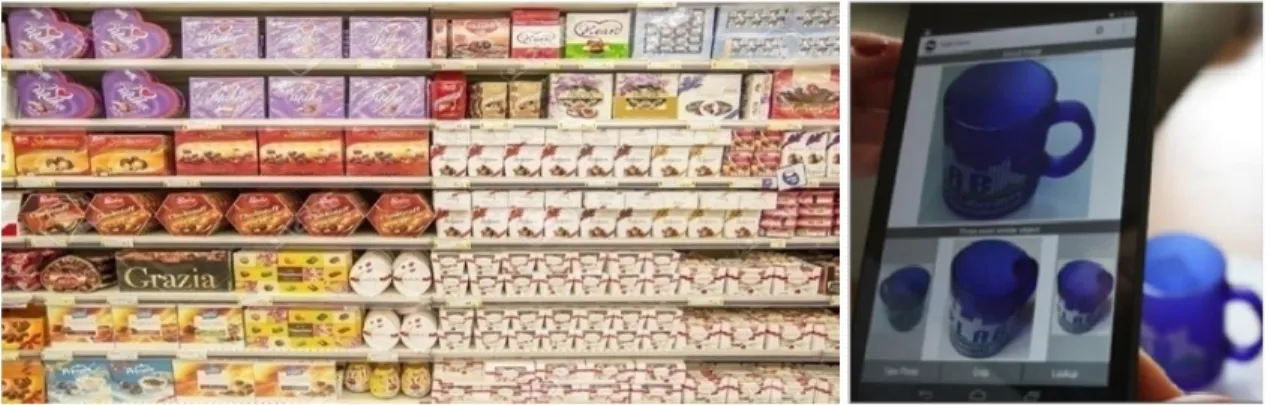
1.1 Real-life recognition examples. . . 3
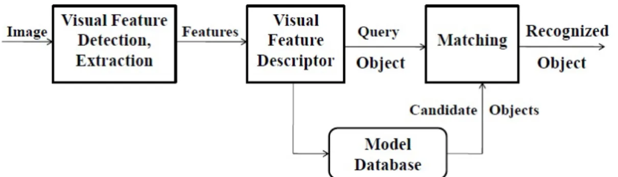
2.1 Basic object recognition flowchart. . . 10
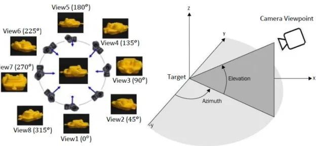
2.2 Model generation setup with target object in the centre. . . 18
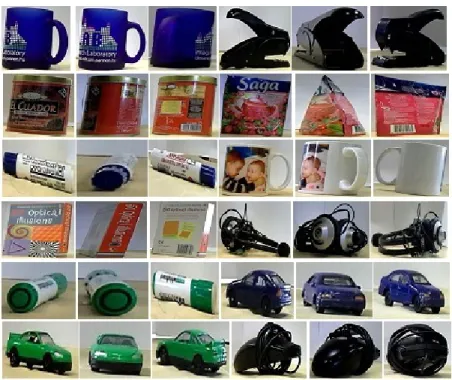
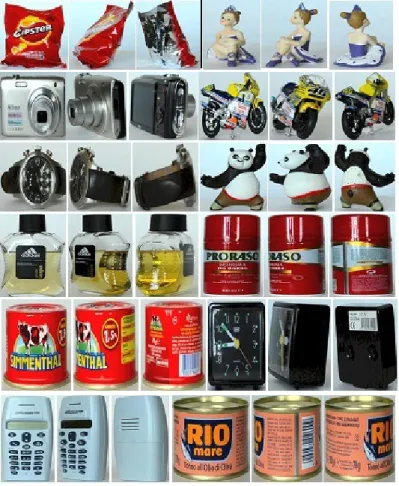
3.1 Test model object examples from the SUP-16 dataset. . . 33
3.2 Test model object examples from the SUP-25 dataset. . . 34
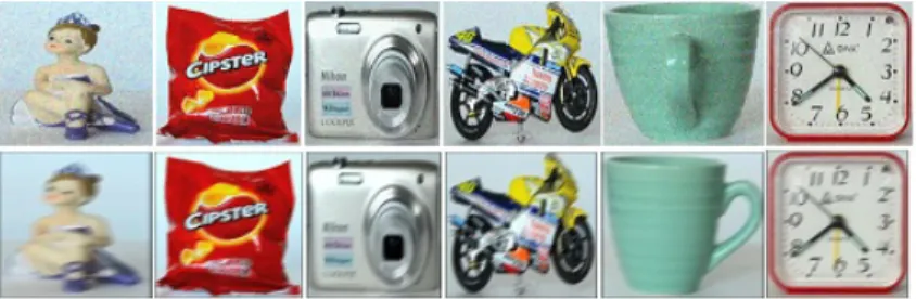
3.3 Top row: examples for the results of tracking. Bottom row: objects and their environment. . . 34
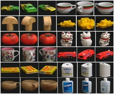
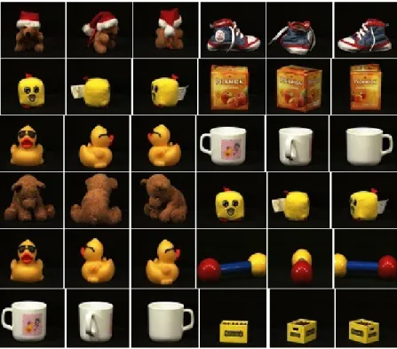
3.4 Test object examples from the SMO dataset with uniform background. 35 3.5 Test model object examples from the COIL-100 dataset. . . 36
3.6 Test model object examples from the ALOI dataset. . . 37
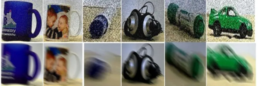
3.7 Noisy and blurred query examples from the SUP-16 dataset. . . 38
3.8 Noisy and blurred query examples from the COIL-100 dataset. . . 38
3.9 Noisy and blurred query examples from the ALOI dataset. . . 38
3.10 Noisy and blurred query examples from the SMO dataset with uni- form background. . . 39
3.11 Noisy and blurred query examples from the SMO dataset with tex- tured background. . . 39
xii
4.1 Illustration of the EIS approach: only the images of the query are compared to the images of the candidates independently. The simi- larity of the query sequence and candidates are based on the sum of Tanimoto Coefficients. . . 42 4.2 Illustration of the VCI approach with three retrieval lists (Nfq=3).
Since C3 was not on L2 but on L1 and L3, C3,4 was added based on T C(qi, cj). . . 44 4.3 The pseudo code for VCI search algorithm. . . 45 4.4 Average hit-rate for query images without distortion (top), with strong
motion blur (middle), and heavy additive Gaussian noise (bottom) for the SUP-16 database. . . 47 4.5 Average hit-rate for query images without distortion (top), with strong
motion blur (middle), and heavy additive Gaussian noise (bottom) for the COIL-100 database. . . 48 4.6 Average hit-rate for query images without distortion (top), with strong
motion blur (middle), and heavy additive Gaussian noise (bottom) for the ALOI database. . . 49 5.1 IMU measurement error distribution. . . 52 5.2 Illustration of the SIIS approach: after finding the best matching
frame of a query and a candidate, other frames are also compared selected on the bases of their similar relative positions as the frames of the query. . . 54 5.3 Average hit-rate for query images without distortion (top), with strong
motion blur (middle), and heavy additive Gaussian noise (bottom) for the SUP-16 database and for VCI ω= 0.5. . . 63
5.4 Average hit-rate for query images without distortion (top), with strong motion blur (middle), and heavy additive Gaussian noise (bottom) for the COIL-100 database and for VCIω = 0.5. . . 64 5.5 Average hit-rate for query images without distortion (top), with strong
motion blur (middle), and heavy additive Gaussian noise (bottom) for the ALOI database and for VCI ω= 0.5. . . 65 5.6 Average hit-rate of the VCI method for motion blur (top) and additive
Gaussian noise (bottom) at different query views (N) and wsettings for the ALOI dataset. . . 66 5.7 Examples for untrained objects, taken from the SMO dataset, to test
recognition performance. . . 68 5.8 Average hit-rate for the SUP-16 dataset with 9 extra untrained queries
with different thresholds. . . 68 5.9 Average hit-rate obtained over the COIL-100 dataset with the VCI Best Match,
VCI W, VCI, AVCI, and with the “Best 10”: queries with motion blur (top); queries with additive Gaussian noise (bottom). . . 71 5.10 Average running time for EIS, SIIS, EIIS, VC and VCI approaches
on a dataset of 100 objects. . . 72 6.1 Geometrical interpretation of transition probabilities. . . 77 6.2 Average hit-rate for query images without distortion (top), with strong
motion blur (middle), and heavy additive Gaussian noise (bottom) for the COIL-100 database. . . 81 6.3 Average hit-rate for query images without distortion (top), with strong
motion blur (middle), and heavy additive Gaussian noise (bottom) for the ALOI database. . . 82
6.4 Average hit-rate for query images without distortion (top), with strong motion blur (middle), and heavy additive Gaussian noise (bottom) for the SMO database with uniform backgrounds. . . 83 6.5 Average hit-rate for query images without distortion (top), with strong
motion blur (middle), and heavy additive Gaussian noise (bottom) for the SMO database with textured backgrounds. . . 84
5.1 Complexity of different approaches atNc = 16,Nfc = 50,Nfleaf = 14, and differentNfq. . . 56 5.2 Comparison of experimental setups of [12] and VCI approach. . . 66 5.3 Average hit-rate for distortion free (DF), motion blur (MB) and ad-
ditive Gaussian noise (GN) with uniform (UB) and textured back- grounds (TB) on the SMO dataset. . . 67 5.4 Hit-rate of VCI with object tracking for SUP-25. . . 69 6.1 Running times in seconds for the retrieval of one object from 100. . . 80
xvi
Introduction
1.1 The Need for New Recognition Methods
The rapid advances in computer techniques, graphics hardware, and networks have led to the wide application of 3D models in various domains, such as 3D graphics, computer aided design (CAD), the medical industry, robot systems, architecture design, and the civil engineering community. Therefore, efficient 3D object retrieval and recognition technologies are of great importance for many applications.
The humans can recognize objects easily without great efforts; on contrary the recognition by machines is one of the fundamental problems of computer vision.
Since childhood, 3D object recognition is one of the most fascinating abilities that humans easily possess. Humans are often able to tell the identity or category despite of the variations of appearance due to change in pose, texture, illumination, defor- mation, or occlusion with a simple glance on a 3D object. Furthermore, humans can easily generalize from observing a set of objects to recognizing objects that have never been seen before.
Machine vision based 3D object retrieval and recognition are basically attempts
1
to mimic the human capability to distinguish different 3D objects. Very similarly to the human brain, deep learning neural networks allow computational models that are composed of multiple processing layers to learn representations of data with multiple levels of abstraction. Convolutional Neural Networks (CNNs) [30] [53] are very often used in image processing giving breakthrough in some visual recogni- tion tasks however, the memory and computational requirements of the application (and training) of such networks is quite large. As the number of embedded and autonomous systems evolves there is a need for new recognition systems, with low power consumption, as alternatives for CNNs. Thus 3D object retrieval and recog- nition techniques need to be developed which are less complex computationally, use less energy, and need limited amount of memory. This gives a motivation for our research.
Optical 3D object retrieval and recognition have many problems in general such as scaling, illumination changes, partial occlusion, and background clutter. In case of capturing 3D objects with mobile devices viewpoint variation and image noise (e.g. motion blur due to hand shaking in poor lighting conditions) can decrease the retrieval and recognition rate significantly. Numerous retrieval and recognition algorithms have been developed, most of them apply single image-based retrieval and recognition. Single view methods may easily fail when there is strong similarity between the captured images or when the background clutter or partial occlusion masks distinctive features. Video based approaches can use more views but suffer from the increased complexity. To avoid big data/cloud processing type of solutions rises a need for efficient lightweight but robust techniques that could run in low cost embedded systems without a high performance back-end support. I. e. our motiva- tion is to develop methods which can retrieve/recognize specific objects viewed from multiple directions. The methods should be relatively fast, require small memory
and easy to extend with new objects (easy to train).
Figure 1.1: Real-life recognition examples.
1.2 Coding Information for Multiple-views with Orientation Sensors
While optical information is crucial for the recognition of 3D objects of the real world, other information, such as depth and audio data (e.g. [38] and [42]) are also often utilized. But besides these, new sensors appeared in the last few years in handheld devices: Inertial Measurement Units (IMUs), which sense either grav- ity, acceleration or orientation, are being embedded into devices more frequently as their cost continues to drop. These devices hold a number of advantages over other sensing technologies: they directly measure important parameters for human interaction e.g., the orientation, position, and motion of cameras and they can easily be embedded into mobile platforms giving low dimensional data.
However, the utilization of these sensors, to help the retrieval and recognition process, is not investigated yet. In this work we build up multi-view object models composed of 2D images with corresponding orientation information. Thus instead
of depth and texture data we use 2D image information and orientation from several viewpoints.
It is obvious that video gives much more visual information about 3D objects than simply 2D projections. As will be discussed later, not only the different views of the objects can be recorded but the 3D structure can be reconstructed by direct [46]
or indirect [75] structure from motion techniques. However, these object centered approaches often require high quality images and camera calibration with relatively large computational power still far from most of the mobile computing platforms and intelligent sensor motes.
1.3 Object Model-centered or Appearance-based Approaches
The 3D object retrieval and recognition methods can be divided into two categories:
(object) model-centered methods and appearance-based or view-centered methods.
Object-centered 3D object retrieval aims to retrieve 3D objects which are repre- sented by 3D models. While these methods compare 3D object information during the search, it is still not straightforward to obtain satisfactory 3D information in several real-world applications, especially when passive optical sensors are used.
Structure from Motion (SfM) [77, 55] is a remote sensing technique that uses multi- ple views of an object to create a three-dimensional set of points, corresponding to the surface, often with associated RGB color values. SfM is often used to reconstruct large spaces ([79]); after georeferencing the point cloud with ground control points, taken with a GPS unit defining the position of recognizable features, the data can be converted to a digital elevation model (DEM). Moreover SfM can be extended with appearance features for recognition purposes [10] and appearance features can be
also used for 3D reconstruction and then for recognition as in [43]. SfM is often used for Simultaneous Localization and Mapping (SLAM) where being real-time can be critical, especially for robotics and unmanned vehicles. In [70] and [25] we have seen that direct SfM can be carried out in real-time with dense data. However, please note that 3D model reconstruction is still computationally expensive and can be un- necessary if our goal is (only) object retrieval and recognition from 2D images. That is we propose that the for the recognition of objects textural and color information, seen from several views, is satisfactory in general. Extending our work with 3D features (such as viewpoint feature histograms - VFHs) or 3D reconstruction could increase the hit-rate. Besides, with the widely spreading active depth acquisition devices (such as Kinect and lidars), it becomes feasible to record color and/or depth information for real objects. These special sensors and the SfM techniques are out of the focus of our research.
The appearance/view-based approach represents objects as collection of 2D views, sometimes called aspects or characteristic views [51], [35]. The advantage of a such approach is that it avoids having to construct a 3D model of an object as well as having to make 3D inferences from 2D features. Many approaches to view-based modeling represent each view as a collection of extracted features, such as extracted line segments, curves, corners, line groups, regions, or surfaces. The success of these view-based recognition systems depends on the extent to which they can extract their requisited features. With real images of real objects in unconstrained environ- ments, the extraction of such features can be unreliable while representing of 3D information in 2D views is not straightforward.
There are several psychophysical supports for two-dimensional view interpolation theory for object recognition in the human visual system. In [13] it is suggested
that the human visual system can be described by recognizing 3D objects by 2D view interpolation. In [27] viewpoint aftereffects also prove that object-selective neurons can be tuned to specific viewing angles in the human visual system. The spatial properties of objects were always considered as significant information in the retrieval and representation of images [15]. View-centered recognition methods can be considered as early machine vision attempts for the recognition of 3D objects.
The idea of storing only a limited number of views of 3D objects and then applying transformations to find correspondence with other views already appear for example in [6] where novel views are generated by the linear combination of stored ones. Rigid objects with smooth surfaces and articulated objects could also be represented this way.
1.4 Contributions
The main contribution of this work is introducing different lightweight algorithms for the retrieval and recognition of a limited number (100-1000) of 3D objects. It is an advantage that the proposed techniques don’t require camera calibration and can be implemented in embedded systems with limited resources (memory and processing power). Moreover, the proposed methods are efficient if the quality of the queries is low, have a built-in mechanism to amend, based on IMU data, possible missing visual information by the insertion of candidates to the evaluation set.
Contrary, it is not the purpose of our work to find the most appropriate visual feature extractors and descriptors. While we apply the Color and Edge Directivity Descriptor (CEDD) [16] [17] as an efficient, fast and low dimensional descriptor our proposed model also could use other popular descriptors (such as SIFT, FAST, GHOST, etc.).
To prove the efficiency of our work several test-beds were used and in order to obtain realistic test scenarios significant motion blur and heavy Gaussian noise was applied on the query images. Besides these simulations we carried out real-life tests where the queries were generated with the help of a semi-automatic process: first the target object was marked by the user then, in the consecutive frames, a mean-shift based algorithm was tracking the object and generating the further query images.
1.5 Thesis Organization
After giving and overview of related papers we define object retrieval and recognition problems and some structures that are used for solving these problems in Chapter 2. In Chapter 3, we describe the various object model datasets and query datasets used in our experimental evaluations. Chapter 4 describes a 3D object retrieval mechanism without using IMU data. This method, using KD-Tree indexing and the Hough transform paradigm, is compared to the approach when all frames of the query are used in an extensive retrieval process.
In Chapter 5, we will show the utilization of IMU data in the Hough paradigm resulting in the increase of hit-rates at relatively fast operation. Besides retrieval, object recognition is presented. Moreover, an application for active perception is also introduced.
Chapter 6 introduces a new 3D object retrieval model by the following mechanisms:
viewer-centric recognition, Markovian estimations, and the fusion of information originating from the visual and orientation subsystems. We have built a Hidden Markov Model (HMM) framework where 2D object views correspond to states, ob- servations are coded by compact edge and color sensitive descriptors, and orientation sensors are used to secure temporal inference by estimating transition probabilities
between states.
Finally, the three theses about the solution of the 3D object retrieval and recog- nition problems, and the list of publications are presented in Chapter 7.
Problem Formulation and Preliminaries
The aim of this chapter, after making an overview of similar techniques, is to de- fine the targeted 3D object retrieval and recognition problems and describe general structures used to solve these problems in later chapters.
2.1 Previous Works
Object recognition is a fundamental task in image processing, still object of research and development for devising automatic solutions. A good broad overview of this topic is well-written in [40]. The general main idea is to find a set of features to describe and discriminate objects of interest from others. A general overview of the process is in Figure 2.1, where first visual features (e.g. lines, corners, edges, color, object shape) are first detected, described, then compared to previously learnt patterns.
Beside this general model Deep Neural Networks (DNN) represent a different approach where feature detection filters and comparison mechanisms are not directly
9
Figure 2.1: Basic object recognition flowchart.
separated [73], [52]. DNN architectures generate compositional models where the object is expressed as a layered composition of primitives. DNNs discover intricate structure in large data sets by using the back propagation algorithm to indicate how a machine should change its internal parameters that are used to compute the representation in each layer from the representation of the previous layer. While DNNs have very high performance for several recognition tasks, they are prone to overfitting because of the added layers of abstraction, which allow them to model rare dependencies in the training data. A key questions with DNNs is training since it needs lots of examples and it is not possible to explicitly define positive or negative rules. To increase its performance the preprocessing of images might be necessary [54]. Also there are alternatives such as Cerebellar Model Articulation Controllers (CMAC) where training can be guaranteed to converge relatively fast [64]. In short: DNNs, and especially CNNs, can be considered as hierarchical, mass feature detectors, which have the power by the combination of large number of various filters. In contrast, we will show that relatively simple features can be used if multiple views are applied and supported with orientation information. Since the feature representation of our approach is much more simple it is very easy to extend our system with new objects. Now we introduce earlier and recent 3D object recognition systems in terms of the types of information they encode and how this
information is organized and used for retrieval by multiple views. Since our approach greatly differs from DNNs we don’t analyze such techniques.
In an early paper of [48] recognition was achieved from video sequences by em- ploying a multiple hypothesis approach. Appearance similarity, and pose transition smoothness constraints were used to estimate the probability of the measurement being generated from a certain model hypothesis at each time instant. A smooth gradient direction feature was used to represent the appearance of objects while the pose was modeled as a von Mises-Fisher distribution. Recognition was achieved by choosing the hypothesis set that has accumulated the maximum evidence at the end of the sequence. Unfortunately, the testing of the method was carried out on four objects only.
In [12] authors created object models, for video object recognition, with the help of SIFT points gathered from images taken by rotating around the object.
Feature points were tracked from frame to frame and video matching was achieved by the comparison of every view of the query with all components of the optimized models of candidates. While the accuracy was about 80% in case of 25 objects, the complexity was too high to be implemented on mobile platforms. Also no explicit technique was utilized to discover the intrinsic structure of sequentially recorded query images and IMUs were not used.
In [61] also SIFT points were used as visual features. The underlying topological structure of an image dataset was generated as a neighborhood graph of features.
Graph pruning was used to get simplified structures and motion continuity in the query video was exploited to demonstrate that the results, obtained using a video sequence, are more robust than using a single image. The ratio of correct retrieval increased to 80% with the method from only 20% of single image queries in case of 100 objects while the complexity was not discussed. Besides using computationally
intensive feature extraction only visual sensors were used in the recognition process.
In [34] in addition to the camera they used the accelerometer and the magnetic sensor to recognize the landscape. Clustered SURF (Speeded Up Robust Features) features were quantized using a vocabulary of visual words, learnt by k-means clus- tering. For tracking objects the FAST corner detector was combined with sensor tracking. Because of the small storage capacity of the mobile device a server-side service was needed to store the large number of images.
Gao et al. [36] proposed a hypergraph learning method for 3D object retrieval, in which the relevance among 3D objects is formulated in a hypergraph structure. In [31] the bag-of-visual-words approach was applied to view-based 3D model retrieval.
Each 3D model was rendered into a group of depth images, and SIFT features were extracted from these depth maps to generate bag-of-features determining the distance between 3D models.
The authors in [4] introduced an Adaptive Views Clustering (AVC) method. In AVC, there are 320 initial views which are captured and representative views are optimally selected by adaptive view clustering with Bayesian information criteria.
A probabilistic method is then employed to calculate the similarity between two 3D models, and those objects with high probability are selected as the retrieval results. There are two parameters in the method, which are used to modulate the probabilities of objects and views, respectively.
In [22] authors proposed a Compact Multi-View Descriptor (CMVD) method, in which 18 characteristic views of each 3D model are first selected through 18 ver- tices of the corresponding bounding 32-hedron. In CMVD, both the binary images and the depth images are taken to represent the views. Then the comparison be- tween 3D models was based on the feature matching between selected views using 2D features, such as 2D Polar-Fourier Transform, 2D Zernike Moments, and 2D
Krawtchouk Moments. For the query object, the testing object rotated and found the best matched direction for the query object. The minimal sum of distance from the selected rotation direction was calculated to measure the distance between two objects.
HMMs are often used in different recognition problems such as speech, musical sound, or human activity recognition but we relatively rarely meet them in the recognition of 2D or 3D visual objects. This is natural since ordered sequences of features are needed to construct HMM models. In [45] affine invariant image features are built on the contours of objects, and the sequence of such features are fed to the HMM. This approach is interesting but seemed to be too unnatural to have later followers. Another approach was proposed in [41], where range images are modeled using HMMs and Neural Networks, using 3D features such as surface type, moments and others.
In [24] authors presented an approach for face recognition using Singular Values Decomposition (SVD) to extract relevant face features, and HMMs as classifier. In order to create the HMM model the 2 dimensional face images had to be transformed into 1 dimensional observation sequences. For this purpose each face image was divided into overlapping blocks with the same width as the original image and a given height, and the singular values of these blocks were used as descriptors. A face image was divided into seven distinct horizontal regions: hair, forehead, eyebrows, eyes, nose, mouth and chin forming seven hidden states in the Markov model. While the algorithm was tested on two standard databases, the advantage of the HMM model over other approaches was not discussed.
The method of Torralba et al. [74] seems to be more close to a real-life temporal sequence: HMM was used for place recognition based on the sequences of visual observations of the environment created by a low-resolution camera. It was also
investigated how the visual context affects the recognition of objects in complex scenes.
In [23] a HMM was used to model the sequence of 2D views gathered from a moving camera, where each view was described using contour-based features. It seems to be a drawback that the contour of the object, often difficult to detect, was employed to compute features, discarding important information such as texture and colors. A thorough experimentation with a standard database is missing, and occlusions were not considered.
The most similar viewer-centered HMM based 3D object retrieval method to ours (described in Chapter 6) was published by Jain et al. [47]. However, there are many differences to our work and there are many ambiguous details in [47]: it is not clear how the crucial emission and transition probabilities were estimated and also the dimension of the applied image descriptor seems to be too small for real-life applications. The dataset in their tests included only gray-scale computer generated images without texture and no orientation sensor was used during the recognition.
Generally speaking the problem of using HMMs in 3D object recognition (espe- cially with handheld devices) is that the transition between states is greatly deter- mined by the user and can not be easily put into the HMM models of objects. To avoid this problem we use orientation sensors to estimate the transition probabilities.
2.2 General Problem Formulation
3D objects form an important type of data with many application domains such as CAD engineering, robotics, visualization, cultural heritage, and entertainment.
Technological progress in acquisition, modeling, and dissemination of 3D geometry leads to the accumulation of large repositories of 3D objects. Let us now introduce
the definition of the 3D object retrieval and recognition problems in the field of computer vision. Please note, that our purpose is to recognize specific objects in contrast to the generic recognition of object categories ([40]).
The 3D object recognition problem can be defined as a labeling problem based on (multiple) views and on known specific models of given rigid 3D objects. An image or images containing one 3D object of interest (and background) and a set of labels, corresponding to a set of models known to the system, is given. We should assign the correct label to regions, or a set of regions, in the images. The 3D object recognition problem is basically accomplished by matching visual features of a query image or query images and of models of possible objects.
The architecture of our 3D object recognition system (as shown previously in Figure 2.1) must have the following components to perform the task:
• Visual Feature Detection and Extraction. Visual feature is some visu- ally observable attribute of the 3D object that will be used in describing and recognizing in relation to other objects. Size, color, texture, and shape are some commonly used features. The feature detection and extraction applies operators to identify locations and measure features that help in forming 3D object hypotheses. The following properties are important for utilizing a good feature detector in computer vision applications:
– Robustness and repeatability: the feature detection algorithm should be able to detect the same feature locations independent of scaling, rotation, shifting, radiometric deformations, compression artifacts, and noise.
– Distinctiveness: the features should be able to show difference between different objects.
– Efficiency: the feature detection algorithm should be able to detect fea-
tures quickly (for the sake of real-time applications) and should use lim- ited amount of memory.
– Quantity: the feature detection algorithm should be able to detect all or most of the important features in the image. The cover of the object is not always satisfactory, especially occlusion can cause considerable problems.
• Visual Feature Descriptor. Feature descriptors encode feature information into a series of numbers and act as a sort of numerical “fingerprint” that can be used to differentiate one feature from another. Ideally this information would be invariant under image transformation, so we can find the feature again even if the image is transformed in some way. The efficient feature descriptor must have several advantages, e.g., small size, low computational cost, easy to compare, suitable for use in large image datasets and insensitive to blur, color distortion and geometrical distortions.
• Visual Feature Matching. Once we have extracted features and generated their descriptors from two or more images, the next step is to establish fea- ture matching between these images. Some transformation invariance can be achieved also with the matching process itself. The complexity of matching can have a great effect on the running time, that is why indexing techniques are often used.
• Model Database. Object representations must be suitable for use in object recognition under various conditions, which means that there must be some potential correspondence between the trained representations and the features that can be extracted from a query. In general the conditions under which the models are built are better than those of making queries.
In our approach 3D object retrieval is the process where a query is initiated by a
user within a collection of 3D objects and a retrieval system responds to the query by presenting a list of retrieved objects sorted in decreasing similarity to the query, according to a predefined measure of object similarity. Each 3D model is represented by a group of 2D views, in several cases also the view’s relative orientation is also given. How to perform multiple view matching is the key topic in view-based 3D model retrieval tasks.
2.3 View-Centered Retrieval and Recognition
Our view-centered representations model the outlook of objects as captured from different viewpoints. Since objects can look very differently from different viewing directions image feature descriptors, the storing database, the search mechanism, and the feature similarity measure should be carefully designed to minimize the amount of data space, retrieval time and to maximize the hit-rate of recognition and retrieval.
Figure 2.2 illustrates the view-centered approach where multi-view object models are built up from 2D images taken from different orientations and being the object of interest in the focus of the camera. To get a complete object model a larger number of different Azimuth and Elevation angles are required. However, for average applications the elevation can be limited (in our tests we used only one elevation angle typical for an object placed on the table).
Why the term recognition is often used generally in our context we can find the difference between recognition and retrieval based on the output of the process: in case of retrieval we know that the target object must be one of the candidates while in case of recognition a previously unknown object can also be targeted. I.e. in the later case we should have the possibility to reject the query as none of those known
Figure 2.2: Model generation setup with target object in the centre.
from previous training.
2.4 Visual Features
In this section we discuss the visual features used in our framework. As mentioned above, there are four main aspects of choosing the right features for a specific image retrieval task: to carry enough information to distinguish images; to be invari- ant to possible distortions; to cover enough area; to be subject of fast and robust comparisons. More precisely there are the following aspects to consider: robust- ness, invariance, repeatability, efficiency, accuracy, quantity, locality, distinctive- ness. Previously (see [21] and [20]) we investigated different types of descriptors in real-life circumstances: MPEG-7 based methods (MPEG7 CLD, MPEG7 EHD, MPEG7 SCD, MPEG7 Fusion); local feature based methods (SURF, SURFVW [16], SIFT); Compact Composite Descriptors [16] [17] (Compact CEDD, CEDD, Com- pact FCTH, FCTH, JCD, CCD Fusion, Compact VW); and others (Tamura texture descriptor, Color Correlogram and Correlation (ACCC) [76], MPEG7-CCD Fusion
[17]). We found two main effects that could seriously degrade the performance of image descriptors in real-life conditions: the change in appearance of colours under different lighting conditions and colour balance settings, and the loss of contrast due to motion blur typically occurring when the image is taken under low lighting conditions with a handheld camera. Detailed descriptions and results of those tests are available in [21] and [20]. Contrary to the popularity of SIFT (and similar de- scriptors in its family such as SURF) in image retrieval we found serious drawbacks such as running time, touchiness to blur and high dimensionality. CEDD was found one of the most robust, fast and compact among those. In [21] and in [20] it is showed that CEDD is quite tolerant for different noises and can be computed fast in today’s mobile platforms. Since then new descriptors were developed, [57] and [69]
give good overviews and analysis about many of them. However, since our purpose was to develop lightweight methods we did not change our decisions to test new alternatives, the very compact CEDD was used in all of our tests. However, we emphasize that other descriptors are also subject to be used since the framework defined in Chapter 4, 5 and 6 could be used with other visual features.
CEDD [16] is a block-based approach where each image block is classified into one of 6 texture classes (non-edge, vertical, horizontal, 45-degree diagonal, 135-degree diagonal, and nondirectional edges) with the help of MPEG7 EHD (Edge Histogram Descriptor). Then for each texture class a 24 bin color histogram is generated where each bin represents colors obtained by the division of the HSV color space. The values of the generated histogram of length 6x24 are then normalized and quantized to 8 bits. Besides its robustness and compactness, however, we should note that there are two disadvantages of CEDD compared to some other popular local point descriptors:
• in its original form it is not rotation invariant;
• as it is a global (area-based) descriptor it needs proper area selection for the target.
The first issue can be handled with a proper similarity measure (see Section 2.6), the second can be fulfilled with manual or automatic segmentation methods. While in our recent application and tests a bounding rectangle around the target was designated manually (or rather the camera was moved to have the object within a bounding box), a good choice for an automatic method could be the Grabcut algorithm known from [67]. It is clear that there are always newer and better global and local descriptors (for overviews see [57] and [69]), the selection of the most appropriate one is out of focus of this thesis.
2.5 Feature Indexing Using KD-Tree
To support the fast search of candidates there are two class of approaches: tree indexing and hashing algorithms. Index structures, containing pointers to descriptor data, are structures to speed up information retrieval and are typically built up off-line. KD-Tree is an efficient data structure, established by Friedman, Bentley, and Finkel [29], [71] and is often used for fast indexing and retrieval. KD-Tree is defined as a binary tree in which every node is a k-dimensional point. Every non-leaf node can be thought of as implicitly generating a splitting hyperplane that divides the space into two parts, known as half-spaces. Points to the left of this hyperplane are represented by the left subtree of that node and points right of the hyperplane are represented by the right subtree. Given a set of N dimensional vectors to be represented, KD-Tree is constructed as follows. First, compute the mean and variance at each dimension of the set, then find the coordinate with the biggest variance and compute the mean at this dimension. Non-leaf nodes divide the set
into two parts known as left subtree (LS) and right subtree (RS). LS contains only the vectors which are smaller or equal to M at the coordinate of highest variance and RS otherwise. Leaf nodes contain those sets which are not divided further. The search is sequential among the elements of leaf nodes.
In [3] authors improved the KD-Tree for a specific usage: indexing a large number of SIFT and other types of image descriptors. They also extended priority search to search among multiple trees in a simultaneously way. In [2] parallel KD-Trees were explored for ultra large scale image retrieval in databases containing dozens of millions of images. In this thesis we also use KD-Tree, however, the number of candidate views (typically below 100,000) does not require the use of such multiple tree solutions.
Recently, product quantization (PQ) [49] and its extensions are popular and successful approximated nearest neighbor search (ANN) methods for handling large- scale data. Each database vector is quantized into a short code, which we call a PQ- code. The search is conducted over the PQ-codes efficiently using lookup tables.
The essence of product quantization is to decompose the original high-dimensional space into the Cartesian product of a finite number of low-dimensional subspaces that are then quantized separately. Optimal space decomposition is important for the performance of ANN search, but still re-mains unaddressed. In general, PQ based approaches consist of the following three main steps: (1) a robust proposal mechanism is used to identify a list of nearest neighbor candidates in the database, (2) a re-ranking step then sorts these candidates according to their ascend- ing approximate distances to the query vector. Finally, the approximated k-nearest vectors after re-ranking are further sorted using an exact distance calculation . In [78] the authors presented an extension to the family of PQ methods called the Product Quantization Tree (PQT). The main contributions of this approach are:
a two level product and quantization tree that requires significantly fewer exact distance tests than prior work; a relaxation of the algorithm for an effective bin traversal order; a fast, re-ranking step to approximate exact distances between query and database points in constant time O(P), where a query vector is split into P parts;
and a highly optimized GPU based open-source implementation.
2.6 Image Similarity Measure
The similarity between two CEDD descriptor vectors is efficiently given with the help of the Tanimoto Coefficient [16]. Let qi be the descriptor of the ith view from the query and cj be the descriptor of the jth view of a candidate. The Tanimoto coefficient is then:
T C(qi, cj) = qTi cj
qTi qi+cTjcj−qiTcj (2.1) where qiT is the transpose vector of the descriptor qi. In case of absolute con- gruence of the vectors, the Tanimoto coefficient takes the value 1, while in case of maximum deviation the coefficient tends to 0. The Tanimoto coefficient was found to be preferable to the similarity functionsL1 (Absolute),L2 (Euclidean Distance) [63]
because of better performance in retrieval tasks. The difference of CEDD vectors is:
T(qi, cj) = 1−T C(qi, cj) (2.2) We need a modified Tanimoto coefficient to achieve rough rotation invariance:
T CR(qi, cj) = max
roll T C(qi,roll, cj) (2.3)
whereroll∈ {0◦,45◦,90◦,135◦}andqi,rollmeans that orientation specific texture
class positions are shifted within the CEDD vector of the query. (Please note, that the extraction of CEDD descriptor values should not be changed, only comparisons take more time to fit the actual candidate cj best).
Please note, that since objects have different appearances from different direc- tions, they will be represented with several frames and the corresponding descrip- tors. These will be denoted such cj,f (that is descriptor of frame f of object j).
Reasonably for queries we use only one index to denote the view.
2.7 The Hough Transformation Paradigm
In this section we discuss the Hough transform method since it will be used as the framework for the combination of weak classifiers. Originally, the Hough transform is a technique which can be used to isolate features of a particular shape within an image. Because it requires that the desired features be specified in some parametric form, the classical Hough transform is most commonly used for the detection of regular curves such as lines, circles, ellipses, etc. but it is also known to be used for object detection [32], object tracking [33] and action recognition [14]. The authors in [5] generalized the classical Hough transform in fuzzy set theoretic framework, called fuzzy Hough transform, in order to handle the imprecise shape description.
In [56] a discriminative Hough transform based object detector is presented where each local part casts a weighted vote for the possible locations of the object center.
The weights can be learned in a max-margin framework which directly optimizes the classification performance and improved the Hough detector. In [66] the circu- lar Hough transform is used to detect the presence of circular shapes and in [72]
authors also used the Hough transform to improve the detection of low-contrast circular objects. Considering the basic approach for detection, the main advantage
of the Hough transform technique is that it is tolerant for gaps in feature boundary descriptions, it is not strongly affected by occlusion in the image and it is also rela- tively unaffected by image noise.
In general there are three main steps of retrieval in this framework:
1. Feature extraction: visual, depth or other observation data can be used to generate descriptors (di ∈D) to gather information about a space/time event or object.
2. Voting: each occurrence of a descriptor votes for a candidate ci with a weight Θ(ci, di). In many cases the weights are determined by training and their value can also depend on different factors (such as the observation’s distance from the candidate or reliability).
3. The Hough Score for a candidate is given:
H(ci) = X
di
Θ(ci, di), (2.4)
and the retrieval is done by selecting the object with the highest score:
ˆ
c= arg max
i H(ci). (2.5)
In our approaches di will be the CEDD descriptors and IMU data (the role of IMUs will be described in details in Chapter 5) .
2.8 Hidden Markov Models
Hidden Markov Models (HMMs) are statistical frameworks in which the system being modeled is assumed to behave as a Markov process with directly unobservable
(hidden) states. An HMM can be considered as the simplest dynamic Bayesian network. The logic behind HMMs was already introduced in the late 1960s and early 1970s in the works of [7], [8]. A HMM is a probabilistic model, which originates from discrete first-order Markov processes.
In this section we briefly overview the theoretical background of HMMs and some related problems. Let S = {S1,· · ·, SN} denote the set of N hidden states of the model. In each t index step this model is described as being in one qt ∈ S state, where t = 1,· · ·, T. Between two steps the model undergoes a change of state according to a set of transition probabilities associated with each state. The transition probabilities have first-order Markov property, i.e.
P(qt=Si|qt−1, qt−2 =Sk,· · ·) =P(qt=Si|qt−1 =Sj) (2.6) Furthermore, we only consider the processes, where the transitions of Equation 2.6 are independent of time. Thus we can define the set of transition probabilities in the form
aij =P(qt =Si|qt−1 =Sj) (2.7) where i and j indices refer to states of HMM, aij ≥ 0, and for a given state PN
j=1aij = 1 holds. The transition probability matrix is denoted byA={aij}1≤i,j≤N. We also define the initial state probabilities:
πi =P(q1 =Si) (2.8)
andπ ={πi}1≤i≤N. Now we extend this model to include the case, where the obser- vation is a probabilistic function of each state. Let O ={o1, o2,· · ·, oT} denote the set of observation sequence. The emission probability of a particular ot observation
for state Si is defined as
bi(ot) =P(ot|qt =Si) (2.9) The set of all emission probabilities is denoted by B ={bi(·)}1≤i≤N. The com- plete set of parameters of a given HMM is described by λ = (A,B, π). A more comprehensive tutorial on HMMs can be found in [65].
2.8.1 Discrete Density HMMs (DHMM)
In case of discrete HMMs we assume that the observation sequences are symbols from a discreteV ={v1,· · ·, vM}alphabet. The symbols correspond to the physical output of the model. In this case the emission probability for a given ot = vk
observation is
bi(ot) =P(ot =vk|qt =Si) (2.10) The B set of emission probabilities can easily be implemented as a 2-D array of size N ×M.
2.8.2 Continuous Density HMMs (CHMM)
Many applications have to work with continuous signals, and Gaussian Mixture Model (GMM) is a widely used representation of the emission probability. In this work we use GMM emission probabilities only, which is defined as
bi(ot) =
M
X
m=1
ωmN(o|µm,Σm) (2.11)
where M is the number of mixture components.
2.8.3 HMM Problems
There are three fundamental problems of interest that must be solved for HMM to be useful in some applications. These problems are the following:
• Evaluation problem. Given an HMM λ = (A,B, π) and an observation sequence O = {o1, o2,· · ·, oN}, determine the probability that model λ has generated observation sequence O, i.e. P(O|λ).
• Decoding problem. Given an HMM λ = (A,B, π) and an observation sequence O = {o1, o2,· · ·, oN}, calculate the most likely sequence of hidden states that produced observation sequenceO.
• Learning problem. Given some training observationO ={o1, o2,···, oN}and general structure of HMM (number of hidden and visible states), determine HMM parameters λ= (A,B, π) that best fit training data.
2.8.3.1 Solution to Evaluation Problem using Forward-Backward Algo- rithm
The Forward-Backward algorithm [50] uses two auxiliary variables for the parameter estimation. First, the forward αt(i) and backward βt(i) variables are calculated inductively as follows.
• Forward Algorithm. The forward variableαt(i) = P(o1, o2,· · ·, ot, qt=Si|λ) is the probability of observing the partial sequence o1, o2,· · ·, ot such that the state qt is Si.
1. Initialization:
α1(i) = πibi(o1) (2.12)
2. Forward recursion:
αt+1(i) =bj(ot+1)
N
X
i=1
αt(i)aij, 1≤j ≤N (2.13) From the definition of Equation 2.12 and 2.13 it is obvious that
P(O|λ) =
N
X
i=1
αT(i) (2.14)
• Backward Algorithm. The backward variableβt(i) = P(ot+1, ot+2,···, oT, qt= Si|λ) is defined similarly, and is the probability of observing the partial se-
quence fromt+ 1 toT, given state Si att.
1. Initialization:
βT(i) = 1 (2.15)
2. Backward recursion:
βt(i) =
N
X
i=1
βt+1(j)aijbj(ot+1), 1≤i≤N, t=T −1,· · ·,1 (2.16) From the definition of Equation 2.15 and 2.16 it is obvious that
P(O|λ) =
N
X
i=1
β1(i). (2.17)
2.8.3.2 Solution to the Decoding Problem using Viterbi Algorithm
The problem of many real-world applications is to efficiently determine the most probable state sequence given an observation sequence O, i.e. we want to find the sequence, which maximizes P(Q, O|λ). We can use the Viterbi algorithm [28] to
find the state sequence. The variable δt is the maximum probability of producing observation sequence o1, o2,· · ·, ot when moving along any hidden state sequence q1, q2,· · ·, qt−1 and getting into qt=Si, i.e.
δt(i) = maxP(q1, q2,· · ·, qt =Si, o1, o2,· · ·, ot|λ) (2.18) and can be calculated inductively as
1. Initialization:
δ1(i) = πibi(o1), 1≤i≤N (2.19) 2. Recursion:
δt+1(j) = max
i [aijbj(ot+1)δt(i)], 1≤j ≤N (2.20) Finally, choose best path ending at T, i.e.
P∗ = max
i [δT(i)]. (2.21)
2.8.3.3 Solution to the Learning Problem using Baum-Welch Algorithm
The most conundrum problem of HMMs is to determine the model parameters which maximizes the probability of a given observation sequence. The Baum-Welch method [7], [8] is an iterative procedure to estimate model parameters that maximum the likelihood P(O|λ). There are three main steps of Baum-Welch algorithm:
• Calculate γt(i) which is the probability of being in state si at index t given the observation sequence O and the parameters λ.
• Calculate ξt(i, j) which is the probability of being in state si and sj at index t and t+ 1, respectively given the observation sequence O and parameters λ.
• Using the above formula γ and ξ, one can re-estimate model parameters.
2.9 Object Tracking
Object tracking is one of the key tasks in the field of computer vision when process- ing a sequence of images. Tracking is the estimation and analysis of trajectories of objects in the plane of the image by moving through a sequence of images. Various methods of object tracking are available, we only mention one, used in our applica- tions later, which can be used with limited resources in real-time applications.
The Meanshift algorithm is designed for static distributions. The method tracks targets by finding the most similar distribution pattern in a frame sequences with its sample pattern by iterative searching. It is simple in implementation, but it fails to track the object when it moves away from camera [80] due to changes in scale.
Continuous adaptive Meanshift (Camshift) easily overcomes this problem. The principle of the Camshift, based on the Meanshift algorithm, is given in [60], [81], [26]. Camshift is able to handle the dynamic distribution by adjusting the size of the search window for the next frame based on the zeroth moment of the current distribution of images. This allows the algorithm to anticipate the movement of objects and quickly track the object in the next frame.
2.10 Summary
In this chapter we discussed the general concepts and tools we use for 3D object retrieval and recognition. We proposed compact visual features and descriptors and
the method to measure the similarity between them. We also discussed the Hough transform paradigm, the concept of Hidden Markov Models, and a tracking method which will serve as the basis for the retrieval mechanisms.
In Chapter 3 we introduce the different types of the 3D object model datasets and queries that are used in our experimental evaluations.
Datasets and Test Issues
The evaluation of object recognition methods greatly depends on the test data and the testing environments itself. As our purpose is to develop methods to recognize small sized 3D objects in real-life conditions, we created different datasets based on our own images or others’ image collections.
3.1 Object Model Datasets
Object models are formed by images taken under good viewing conditions. Each object is captured from several views but the same elevation. These data can be considered as training information for the knowledge base of the recognition mech- anisms. We introduce five separate object model datasets, with different size and visual nature. There are several reasons that besides standard datasets we used our own recordings (SUP datasets). Orientation data was precisely given for the stan- dard datasets. Using our IMU sensor (with possible inaccuracy) is more realistic in experimental tests. To make tracking experiments was not possible with online datasets, thus new samples (in SUP-25), with several other visible objects, were necessary.
32
3.1.1 SUP-16 Dataset
SUP-16 is a small dataset including 16 objects, where 44-73 views per object were captured from the same elevation but from different azimuth leading to approxi- mately 900 images. Objects were centered and a bounding box was manually de- fined for each image. Image sizes and side ratios varied a lot as shown in Figure 3.1.
As we can see the object size, shape, color, contrast can vary from view to view.
Some view of the same object can be very different from the other (see f.e. the green pencil or the white cup). The background of the objects were only roughly uniform and the surface of objects was sometimes glossy.
Figure 3.1: Test model object examples from the SUP-16 dataset.
3.1.2 SUP-25 Dataset
The SUP-25 dataset, illustrated in Figure 3.2, includes 25 different objects, where 64-77 images of each object were recorded from different views at the same elevation
leading to approximately 1800 images. This dataset was created by our tablet to test the VCI approach with automatic Camshift tracking applied for the generation of queries (described in Section 5.5.4). Figure 3.3 illustrates some tracked windows and the environment of the objects.
Figure 3.2: Test model object examples from the SUP-25 dataset.
Figure 3.3: Top row: examples for the results of tracking. Bottom row: objects and their environment.
3.1.3 SMO Dataset
The SMO dataset [12], illustrated in Figure 3.4, includes 25 different objects with uniform background, where 36 images of each object were recorded by rotating the object in the plane at 10◦ steps leading to approximately 900 images. This database is chosen for comparison with the method of [12].
Figure 3.4: Test object examples from the SMO dataset with uniform background.
3.1.4 COIL-100 Dataset
The COIL-100 dataset [59] includes 100 different objects. The objects were placed on a motorized turntable against a black background, 72 images of each object