deposition of atmospheric aerosol particles
Cite as: Chaos 29, 071103 (2019); https://doi.org/10.1063/1.5110385
Submitted: 16 May 2019 . Accepted: 21 June 2019 . Published Online: 16 July 2019 T. Haszpra
COLLECTIONS
This paper was selected as Featured
ARTICLES YOU MAY BE INTERESTED IN Symmetry induced group consensus
Chaos: An Interdisciplinary Journal of Nonlinear Science 29, 073101 (2019); https://
doi.org/10.1063/1.5098335
Recurrence network analysis of exoplanetary observables
Chaos: An Interdisciplinary Journal of Nonlinear Science 29, 071105 (2019); https://
doi.org/10.1063/1.5109564
Hyperchaos and multistability in the model of two interacting microbubble contrast agents Chaos: An Interdisciplinary Journal of Nonlinear Science 29, 063131 (2019); https://
doi.org/10.1063/1.5098329
Intricate features in the lifetime and deposition of atmospheric aerosol particles
Cite as: Chaos29, 071103 (2019);doi: 10.1063/1.5110385 Submitted: 16 May 2019·Accepted: 21 June 2019·
Published Online: 16 July 2019 View Online Export Citation CrossMark
T. Haszpra
AFFILIATIONS
Institute for Theoretical Physics and MTA–ELTE Theoretical Physics Research Group, Eötvös Loránd University, Budapest H-1117, Hungary
ABSTRACT
The advection of particles emanated, e.g., from volcano eruptions or other pollution events exhibits chaotic behavior in the atmosphere. Due to gravity, the particles move downward on average and remain in the atmosphere for a finite time. The number of particles not yet deposited from the atmosphere decays exponentially after a while characteristic to transient chaos. The so-called escape rate describes the rapidity of the decrease, the reciprocal of which can be used to estimate the average lifetime of the particles. Based on measured wind field data, we fol- low aerosol particles and demonstrate that the geographical distribution of the individual lifetime of the particles distributed over the globe at different altitudes shows a filamentary, fractal distribution, typical for chaos: the lifetime of particles may be quite different at very nearby geographic locations. These maps can be considered as atlases for the potential fate of volcanic ash clouds or of particles distributed for geo- engineering purposes. Particles with similar lifetime deposit also in filamentary structures, but the deposition pattern of extremely long-living particles covers more or less homogeneously the Earth. In general, particles emanated around the equator remain in the atmosphere for the longest time, even for years, e.g., for particles of 1µm radius. The escape rate does not show any considerable dependence on the particles’
initial altitude, indicating that there exists a unique chaotic saddle in the atmosphere. We reconstruct this saddle and its stable and unstable manifolds on two planar slices and follow its time dependence.
© 2019 Author(s). All article content, except where otherwise noted, is licensed under a Creative Commons Attribution (CC BY) license (http://creativecommons.org/licenses/by/4.0/).https://doi.org/10.1063/1.5110385
Pollutant particles emitted during volcano eruptions or from anthropogenic sources like industrial accidents sooner or later leave the atmosphere and deposit on the ground. We show that the lifetime of individual particles has a broad distribution, and its geographical distribution displays a time-dependent, filamen- tary structure often with even a tenfold difference between very nearby particles. The deposition pattern on the ground is also found to be filamentary, characteristic to chaotic dynamics. We show that the trajectories of nearby particles with similar life- times remain close to each other for long times and they deposit at nearby locations. The boundary among these types of coherent particle groups can be considered to form repelling Lagrangian Coherent Structures. The rate of the exponential decrease of long- living particles does not change with the initial altitude but shows a quadratic dependence on the particle size.
I. INTRODUCTION
Everyday news often report on atmospheric hazards due to volcanic ash clouds or pollutants emanated from industrial accidents.
Not only their atmospheric residence but also the deposition of these materials on land and ocean territories may result in environmen- tal or health risk. The most known recent pollution events include, e.g., the 2010 eruptions of the Eyjafjallajökull volcano which caused airspace closures across Europe as its volcanic ash clouds reached even the Iberian Peninsula1and Italy,2,3thousands of kilometers away from Iceland; the 2011 eruption of Grímsvötn whose ash cloud cov- ered some part of Scandinavia and Greenland;4,5and the Fukushima Daiichi nuclear disaster as a result of which radioactive materials were transported in the atmosphere over the Pacific Ocean6–8travel- ing around the Northern Hemisphere within a few weeks producing measurable concentration even in Europe.9–14
In three-dimensional flows, as is the case for the atmosphere, the advected particles typically exhibit chaotic behavior: nearby par- ticles diverge within short time, their motion is irregular, and they trace out complicated but well-organized (fractal) structures. The chaoticity of the pollutant advection can be studied by means of different quantities, such as the Lyapunov exponent describing the strength of the trajectory separation of initially nearby particles as well as the local mixing (see, e.g., Refs.15–21) or the topological
entropy22–24characterizing the rate of the exponential stretching of pollutant clouds in the atmospheric context and being closely related to the unpredictability of the spreading and the complexity of the structure of a pollutant cloud.25,26
Due to the vertical component of air velocity and gravity, particles with nonzero mass (e.g., aerosol particles) carry out this complicated, chaotic motion for finite duration because they move downward on average. Their dynamics is transiently chaotic.27How- ever, as the measurements related to the above mentioned eruptions and nuclear accident demonstrate, small particles may travel far away from their initial source around the Earth roaming complicated paths before they deposit on the ground. It is shown in the paper that the time dependence of the number of particles not yet deposited from the atmosphere does not change for a while but then starts to decay rapidly, exponentially. The rate of this exponential decrease is called the escape rate.27–29
In this study, we simulate the motion of individual aerosol par- ticles driven by measured atmospheric winds, downloaded from a meteorological database. We show that particles do not deposit onto the surface as large, coherent patches, but initially close particles may leave the atmosphere at locations that are thousands of kilometers away from each other. We also demonstrate that the geographical distribution of the individual lifetime of the particles shows a fil- amentary, fractal geometry, typical for chaos, i.e., the deposition process is much more complicated than a simple settling with a given terminal velocity, even for identical particles.
We will see that the trajectories of nearby particles with similar lifetimes remain close to each other for long times and they deposit at nearby locations. The boundary among these types of coherent parti- cle groups can be considered to form Lagrangian Coherent Structures (LCS).30–33They form robust skeletons of the particle dynamics. Note that these are 3D LCSs, such as the ones in Refs.34and35, and are formed by particles of finite mass.
The paper is organized as follows. SectionIIprovides a brief overview of the features and concepts of transient chaos. SectionIII introduces the RePLaT model and the equations of motion by which the trajectories of the aerosol particles are determined and describes also the meteorological data and the initial setup of the simulations.
The results for the geographical distribution of the lifetimes, for the escape rate and average lifetime of the particles depending on the par- ticle size and initial altitude, for the particles’ deposition pattern and the chaotic saddle are presented in Sec.IV. SectionVsummarizes the main conclusions of the work.
II. TRANSIENT CHAOS: CHAOTIC SADDLE, LIFETIME, ESCAPE RATE
Chaotic behavior taking place only for a finite duration is called transient chaos.27,28,36In such cases, there exists a nonattracting set with fractal structure in the phase space, called chaotic saddle, which is responsible for the chaotic motion. Trajectories initialized exactly on the saddle would never leave it and carry out chaotic motion for infinitely long time. Nevertheless, as the chaotic saddle is a zero- measure set, in computational simulations using random initial con- ditions, its points can only be reached approximately: trajectories with random initial conditions sooner or later leave any arbitrary environment of the chaotic saddle and, thus, have finite lifetimes.
The rate of the emptying process is measured by the so called escape rate. For passive advection, the phase space is the real space; there- fore, we expect the chaotic saddle to be located in the atmosphere, but since it might move in time, its precise localization is a challenge.
In order to determine the escape rate it is worth initializing a large number of trajectories (n01) in a preselected region and tracking each of them until they escape the given region. We empha- size that after escape they cannot return to the investigated region.
Therefore, the numbern(t)of the trajectories which have not left the region up to time t reduces monotonically. After some time t0—which depends on the initial conditions, the initialization time instant and the properties of the particles—n(t)start to decay rapidly, exponentially,
n(t)∼exp(−κt) ift>t0. (1) Here,κis called the escape rate.27,36,37The larger the escape rate is, the more trajectories leave the preselected region up to a given time instant aftert0, i.e., the faster the escape process is. The range of the individual lifetime of the trajectories can be broad. In general, the quantityκ−1=τavecan be considered to be an estimate of the average lifetime of the typical trajectories aftert0.
In this study, in the context of atmospheric pollutant spreading, trajectories of small aerosol particles of the density of typical vol- canic ash particles are tracked, the preselected region is the entire atmosphere and, because the particles move downward on average, the escape rate provides a measure for “the speed of the deposi- tion process” toward the surface. In systems with irregular time dependence, such as the atmosphere, the chaotic saddles are also time-dependent, which implies also time-dependent escape rates and average lifetimes. The quantities numerically measured in this study shall characterize the saddle in the time interval over which a non- negligible part of the investigated particles stayed in the atmosphere.
In a previous study,29we demonstrated that in the atmosphere, two chaotic saddles with different escape rates coexist, and in this case, the numbern(t)is the sum of the two exponential expressions.27 However, in this paper, we focus only on the chaotic saddle with the smaller escape rate which characterize the escape of particles with longer lifetimes. As a novelty of this study, maps of the geographi- cal distribution of the individual lifetimes are presented, the chaotic saddle is reconstructed, and the relationship with LCSs is revealed.
III. DATA AND METHODS
We consider pollutant clouds consisting a large number of small, heavy spherical particles. The particle trajectories are calculated by the RePLaT (Real Particle Lagrangian Trajectory) atmospheric dis- persion model29,38 taking into account advection and the role of gravity through the terminal velocity of individual particles. Because of their large density and small size, the equation of motion of a par- ticle of velocity vectorvpin a wind fieldv(r,t)is taken in vectorial form to be
vp=v(r,t)+wtermn, (2) wherewterm<0 is a settling velocity andnis a unit vector point- ing upward. Similar types of Lagrangian dynamics are used in the oceanic context in Refs.39–41and in simple atmospheric transport and dispersion models which track the motion of realistic aerosol particles.42,43
We neglect the effect of turbulent diffusivity and the removal of particles by wet deposition (i.e., rain-out or washout by precipitation or clouds) because these effects influence a negligible short period of their lifetime. RePLaT considers the equations of motion in longi- tude–latitude–pressure coordinates fitted to the coordinate system of the utilized meteorological data (described at the end of this section),
dλp
dt =u(λp(t),ϕp(t),pp(t),t)
REcosϕp =urad(λp(t),ϕp(t),pp(t),t), (3a) dϕp
dt =v(λp(t),ϕp(t),pp(t),t) RE
=vrad(λp(t),ϕp(t),pp(t),t), (3b) dpp
dt =ω(λp(t),ϕp(t),pp(t),t)+ωterm(λp(t),ϕp(t),pp(t)), (3c) where λp and ϕp are the longitude and latitude coordinates, pp(t)≡p(λp(t),ϕp(t),pp(t),t)is the pressure coordinate of a parti- cle,RE=6370 km is the Earth’s radius,uandvare the zonal and meridional velocity component of the air in the units of m s−1,urad andvradare the same but in units of s−1fitted to the longitude–latitude coordinates as the right hand side of Eqs.(3a)and(3b)defines,ωis the vertical component in the pressure system, andωtermis the cor- responding terminal velocity of the particle in motionless air of the form of
ωterm=2 9r2ρp
νg2. (4)
Here,randρpare the radius and the density of the particle, respectively,ν is the kinematic viscosity of air, and gdenotes the gravitational acceleration.
The dependence ofνon temperatureTand pressurepis calcu- lated according to Sutherland’s law,44
ν=β0 T3/2 T+TS
RdT
p . (5)
Here,β0=1.458×10⁻⁶kg m−1s−1K−1/2 is Sutherland’s con- stant,TS=110.4 K is a reference temperature, andRd=287 J kg−1 K−1is the specific gas constant for dry air.
As a development compared to the previous model version which uses Euler’s method29,38in this study, RePLaT determines the particle trajectories using the second-order Petterssen scheme with variable time step1tchosen as1t=Cminn
1λ
|urad|;|v1ϕrad|;|ω+ω1pterm|o withC=0.2, where1λ,1ϕ, and1pdenote the grid size in longi- tudinal, meridional, and vertical directions, respectively. By means of such a choice the smallest features resolved by the meteorolog- ical fields are taken into account as pointed out in Ref. 45. The meteorological data are interpolated to the particles’ position using multilinear interpolation in space and time. If a particle crosses the lowest pressure level, it is considered to be deposited, i.e., it con- sidered to be escaped. The density of the particles in this study is chosen to beρp=2000 kg m−3, corresponding to the typical density of aerosol particles of volcanic origin.46–48
The meteorological data required for the trajectory calculation, i.e., theu,v,ω, andTfields in the pressure coordinate system are retrieved from the ERA-Interim reanalysis database of the Euro- pean Centre for Medium-Range Weather Forecasts (ECMWF)49on a 1.5◦×1.5◦horizontal grid with 6 h of time resolution for the pressure levels from 1000 to 100 hPa for the years 2014–2017.
IV. RESULTS
A. Geographical distribution of the lifetime
In order to study the chaotic features of the global particle depo- sition process from the atmosphere and gain an illustrative picture, at first,n0=103×103particles are initialized uniformly distributed at different pressure levels over the globe on 1 January 2016 at 00 UTC.
Particles are tracked until timeτwhen they escape from the atmo- sphere which is defined by the crossing of the 1000 hPa level (as the ground), the lowest boundary of the meteorological data in the study.
Figure 1illustrates that the geographical distribution of the indi- vidual lifetimeτof the particles exhibits an intriguing pattern. Theτ values can be considerably different for particles started even within short (on the order of 10–100 km) distances, see, e.g., the location of yellow and red points in the black rectangle in panel d and its blow up in panel j. Generally, the lifetimes display a fractal-like dis- tribution with larger lifetimes for smaller particles started on higher altitudes. More and more filamentary structures show up including finer scale details along with the decrease of the particles radius and with the moving up of the initialization level. For example, the details of the spiral forms which can be considered as fingerprints of emerg- ing and decaying atmospheric cyclones (e.g., the one in the region [0◦E, 120◦E]×[60◦N, 90◦N]) appear from the mostly smoothed out shape on lower initialization levels to a clearly visible filamentary spiral on the upper levels.
In general, the tropical region possesses the largest lifetimes.
This can be related to the Intertropical Convergence Zone (ITCZ) where the southeast and northeast trade winds converge and strong upward vertical motion is generated to which the warm surface also contributes. The location of the ITCZ follows the annual cycle of solar insolation.50,51This cycle is also manifested in the distribution of life- times: e.g., inFig. 1(d), on 1 January, the red band is largely south to the Equator and it becomes shifted gradually north to the Equa- tor half a year later, on 1 July asFig. 1(k)indicates. The displacement is the most pronounced in the Asian-Australian monsoon region in harmony with ITCZ studies (see, e.g., Refs.52and53).
For large particles initialized on lower levels [e.g.,Figs. 1(f)–1(i)], some spots (likely related to cyclonic upward motions at the begin- ning of the simulation) show similar lifetime values to the ones in the tropics. It is worth noting that the distribution of lifetimes does not characterize merely one single time instant, but it is the result of the history of dynamics, the particles are subjected to during their entire lifetime. Of course, the particles which come to the higher lay- ers of the atmosphere already at the beginning of their atmospheric life (i.e., they are initialized at locations which are characterized by strong upward flows, such as the ITCZ or cyclones) have more chance to live further.
It is worth investigating the fate of initially close particles belonging to the same “color tendril” in the geographical distri- bution of lifetimes (i.e., nearby particles having similar lifetimes), compared to the fate of particles which belong to different tendrils.
In order to gain an impression, we choose nearby particles from the dense filamentary region in the middle ofFig. 1(j), where the ini- tial position of three particle pairs are marked by six black dots.
Figures 2(a)and2(b)illustrate clearly that the trajectories of nearby particles started in regions of the same color tendril keep moving together during their entire lifetime, and the distance between these
FIG. 1. The geographical distribution of the individual lifetimeτof 103×103particles initialized uniformly over the globe at different pressure levels. Initialization time is (a)–(j) 1 January 2016 00 UTC and (k) 1 July 2016 00 UTC. The initial level is (a)–(c) 300 hPa, (d)–(f) 500 hPa, (g)–(i) 700 hPa, and (j)–(k) 500 hPa. The particle radiusr is [(a), (d), and (g)] 5µm, [(b), (e), and (h)] 7µm, [(c), (f), and (i)] 9µm, and [(j) and (k)] 5µm. Panel j is the blow-up of the rectangle in panel d: 103×103particles are initialized in the rectangle [100◦E, 140◦E]×[20◦S, 0◦S] on the 500 hPa level. Black dots indicate the initial location of particles which are tracked inFig. 2.
FIG. 2.(a) At most 13-day-long trajectories of the particles initialized at the black dots inFig. 1(j). Particles initiated in the same region are marked by the shades of the same color and by the same numbers. The legend indicates also the particle’s lifetime in days in the parentheses. Markers are plotted in every 6 h; therefore, the speed of the particles can also be read off. (b) The distance between the different particle pairs (identifiers are indicated in the legend).
particle pairs does not increase in an exponential manner, rather it slightly decreases over several days. However, the distance between initially nearby particles from different color tendrils grows fast, as it is expected for chaotic processes, and the trajectories of east-west separated pairs marked by red, green, blue arrive in quite different locations after 10–13 days, in Indonesia, and the western and central part of the Pacific Ocean, respectively [seeFig. 2(a)]. The distance between the red and green, and the green and blue endpoints, the location of the deposition, is about 2000 and 5000 km, respectively.
Based on these features, even though the geographical distribution of the lifetimes in several regions is continuous, a sharp edge between tendrils of substantially different lifetimes may be considered to be a hyperbolic Lagrangian Coherent Structure (LCS). These are known
FIG. 3. (a) A blow-up ofFig. 1(j)representing the geographical distribution of the particles’ individual lifetimeτ. (b) FTLE calculated from 5-day forward integration.
(c) FTLE calculated from 10-day forward integration. FTLE is not plotted for initial positions where the particles are deposited within the studied time interval.
to be structures correspond to stable manifolds of saddles and are called repelling LCSs in Refs.54and55.
For completeness, in order to detect traditional repelling LCSs, the geographical distribution of the finite-time Lyapunov exponent (FTLE) is determined inFigs. 3(b)and3(c)for a horizontal planar
slice at Indonesia and Northern Australia. These maps show that the ridges of the FTLE map, i.e., the intersections of the LCSs with the planar slice, compose a fractal set of lines. Furthermore, the fil- amentary structure of the FTLE maps is strikingly similar to that of the lifetime distribution in Fig. 3(a) [a blow-up of Fig. 1(j)]
and the ridges in the FTLE coincide with reasonable accuracy with the boundaries of the tendrils inτ. See, e.g., the edge of the large yellow ([122◦E, 130◦E]×[20◦S, 14◦S]) and red ([134◦E, 140◦E]× [20◦S, 13◦S]) triangles in the lower left and lower right corner of Fig. 3(a), respectively, and the corresponding ridges inFigs. 3(b) and3(c). Comparing the structure of the dense filamentary region through Timor and the Timor Sea ([123◦E, 128◦E]×[16◦S, 8◦S]) in the panels ofFig. 3also confirms the association of the LCSs with the boundaries in the lifetime distribution. Thus, all of these suggest that the LCS surfaces (or filaments in planar slices) separate domains from which the particles escape to different escape regions27on the surface.
B. Escape rate and average lifetime
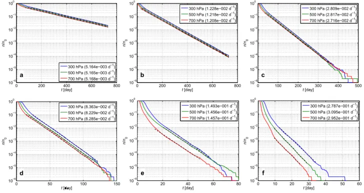
Due to gravity every aerosol particle leaves the atmosphere sooner or later. InFig. 4, the time dependence of the ration/n0of the particles survived in the atmosphere up to timetis shown for dif- ferent initial levels and particle radii. The panels demonstrate clearly that for a certain time interval of lengthtp, a plateau is formed in n/n0 at the value of unity: none of the particles falls out from the atmosphere.
The plateau in each panel ofFig. 4is followed by a short, steep decrease the characteristic time of which is 10–50 days. These seg- ments can be considered to be a result of rather strongly repelling chaotic saddles;29 however, their strong dynamical instability does not allow a statistically reliable estimate to compute the correspond- ing “short-term” escape rates here.
We emphasize that the time interval oft0=10−50 days after which the long exponential decrease starts in the panels coincides with the average time after which the distribution of pollutant clouds generally covers a hemisphere.56Therefore, one can safely assume that the decay of the particles is governed by a global chaotic saddle from this time on.
The slope of then/n0curves, i.e., the escape rateκ, for the time period when the decrease is clearly exponential depends only on the particle radiusrand does not depend considerably on the initial alti- tudepof the particles, asFig. 4shows. This is in harmony with the fact that the escape rate characterizes the deposition dynamics of those exceptional particles which live longer in the atmosphere than most of the particles, and, therefore, they have enough time to forget their initial conditions and become well mixed in the atmosphere before depositing.
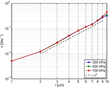
The dependence of κ on r seems to be quadratic as Fig. 5 shows. This is in harmony with the fact that the terminal velocity is a function ofr2, and, additionally, in rough average, the updrafts and downdrafts in the atmosphere balance each other’s effect on the particles resulting on average in their fall with their terminal velocity.
FIG. 4. The ration/n0of particles not escaped the atmosphere up to timet. The particle radiusris (a) 1µm, (b) 2µm, (c) 3µm, (d) 5µm, (e) 7µm, and (f) 9µm. Legends indicate the pressure level on which the particles are initialized with uniform distribution over the globe and the corresponding escape rate in parentheses. Black dashed lines are the fitted linear regression lines to the longest linear regime for the calculation of the escape rate.
FIG. 5. The dependence of the escape rateκon the particle radiusrand the initialization level (see the legend). Black dashed line indicates anr2curve for illustrative purposes.
It is worth investigating the average lifetime of the particles as a function ofr. InFig. 6, this quantity is estimated in three different ways:hτidenotes a simple averaging over the obtained individual lifetime of the particles,τterm is computed assuming that a parti- cle with radiusr, and densityρpfalls in each time instant with its
FIG. 6. The dependence of the estimated average particle lifetimes on the parti- cle radiusrand the initialization level (see the legend).hτidenotes the average of the measured individual lifetimes,τtermis determined as if particles would fall with their altitude-dependent terminal velocity [Eq.(4)], andτaveis estimated based on the escape rate [Eq.(7)]. The variablehτiis plotted only forr≥3µm since forr<3µm not all of the particles leave the atmosphere within the studied two years.
pressure-dependent terminal velocity [Eq.(4)] in motionless air, τterm=
Z p1=1000 hPa p0
dp
ωterm(p). (6)
We note that theτtermcurves follow anr−2law as a consequence of Eq.(4).
In Sec.II, it is mentioned that the average lifetimeτaveof the par- ticles can be approximated byκ−1. However, in our case, the curves ofn(t)/n0consists of three segments: a plateau withn(t)/n0≡1 up totp; a short, steeper decrease betweentpandt0fromn(t)/n0=1 to n(t0)/n0; and a long exponential decrease fromt0on with the expo- nentκ. Assuming an exponential decrease also between the points (tp, 1)and [t0,n(t0)/n0] and estimating its short-term escape rate as κs= −log(n(t0)/n0)/(t0−tp)the average individual lifetime can be estimated as
τave≈tp+ 1 κs
+
t0+1 κ
n(t0) n0
, (7)
wheretpandt0are extracted from the data. The typical values oftp,
1
κs,t0, 1κ, andn(tn0)
0 increase with decreasing particle radius and with increasing initial altitude. The values oftprange from about 0.5–1 days forr≈9−10µm and 700 hPa to 5–10 days forr≈1−2µm and 300 hPa. The same numbers forκ1
sare 1–2 days and 70–170 days, fort07–10 days and 50–120 days, forκ12–3.5 days and 80–190 days, and forn(tn0)
0 0.002 and 0.5, respectively.
Figure 6shows that the measured averagehτiand the two esti- mates τterm and τave for the average lifetime yield similar results, especially forr≥5µm particles. The average lifetime ranges from about 1.5 days to hundreds of days forr=10µm to r=1µm particles. For example, the average lifetime ofr=5µm particles emitted into the middle troposphere (500 hPa) is about 10–15 days.
The difference is the largest fromτterm, which is the result of the fact that the particles do not fall directly purely vertically through the atmosphere from their initial altitude onto the surface with their terminal velocity rather moving on complicated paths before depositing.
C. Deposition pattern
We consider the location of the deposition where a particle hits the surface. It is worth investigating whether the evolving deposition pattern also shows the signatures of chaos. InFig. 7, the deposi- tion pattern is plotted for the particles inFig. 1(j), both for time instants before and during the long-term exponential decay of the particles [vsFig. 4(d)]. It illustrates that even before the long-term transient chaotic behavior occurs, the distribution of the deposited particles is inhomogeneous with filamentarylike structures (blue) around Indonesia and Australia. After the long-term exponential decay begins (cyan), the deposition pattern also consists of several tendrils. We draw attention to the fact that after 20–21 days, the depo- sition pattern of the particle cloud covers a significant part of the Southern Hemisphere and has some extensions also on the North- ern Hemisphere. Plotting the deposited particles for a longer time period during a time interval of the long-term exponential decay, from 40 to 50 days, the pattern is more homogeneous but denser and sparser regions are still observable (red).57 Inhomogeneous
FIG. 7. Deposition pattern in time intervals indicated in the legend for the particles initialized inFig. 1(j).
deposition patterns for the same volume-preserving equation of motion Eq. (2) have recently been observed in oceanic settings and have been explained through stretching (due to advection) and projection (onto the deposition surface) of material layers.40,41,58
D. Chaotic saddle
Here, we show that the chaotic saddle underlying the deposition dynamics in the atmosphere can be reconstructed from our data. We carry out the reconstruction on two planar slices in the atmosphere.
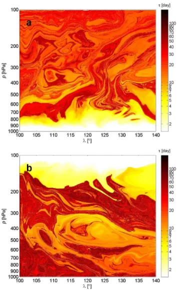
The first row ofFig. 8shows on a 2D horizontal segment, the chaotic saddle and its stable and unstable manifolds forr=5µm particles initialized on the 500 hPa level inFig. 1(j). The second row is a vertical intersect forr=5µm particles initialized atϕ=10◦S in a rectangle of [100◦E, 140◦E]×[1000 hPa, 100 hPa].
The stable manifold at the time instant 00 UTC, 1 January 2016 contains the location of the particles which do not deposit from the atmosphere at all. In practice, one chooses a long time period: we took 50 days here. The unstable manifold at the same time instant consists the end points of trajectories which are started at some earlier time and remained in the atmosphere. The latter manifold is created here by tracking the backward trajectories of the particles initialized at 00 UTC, 1 January 2016 and plotting the initial location of those particles that do not leave the atmosphere (typically in the upward direction) up to 50 days. The chaotic saddle is plotted as the intersect of the stable and unstable manifold. Since it turned out fromFig. 1 that the long-living particles start principally close to the Equator, it is expected that the chaotic saddle is the densest in this region, too.
The vertical intersect shows that the stable manifold generally do not expand down to the surface: for r=5µm particles below approximately the 800 hPa level, the particles have practically no chance to live long in the atmosphere, they are deposited generally
FIG. 8. Horizontal [(a)–(c)] and vertical [(d)–(f)] segments of the stable [(a) and (c)] and unstable [(b) and (d)] manifolds of the chaotic saddle [(c) and (f)] forr=5µm particles initialized on 1 January at 00 UTC. For panels (a)–(c), particles are initialized on the 500 hPa level in a rectangle of [100◦E, 140◦E]×[20◦S, 0◦S]. For panels (d)–(f), particles are initialized atϕ=10◦S in a rectangle of [100◦E, 140◦E]×[1000 hPa, 100 hPa]. The manifolds are approximated by plotting the particles remaining in the atmosphere for at least 50 days in forward (stable manifold) and backward (unstable manifold) simulations and both in the backward and forward simulations (saddle).
The red line in panels (a)–(c) and (d)–(f) indicates the latitude (altitude) along which the vertical (horizontal) segment in panels (d)–(f) and (a)–(c) is taken.
FIG. 9.A vertical intersection of the distribution of individual lifetimesτ in a forward (a) and backward (b) simulation. Particles ofr=5µm are initialized uniformly in the rectangle [100◦E, 140◦E]×[1000 hPa, 100 hPa] at 10◦S on 1 January 2016 at 00 UTC.
within 3–4 days [seeFig. 9(a)]. For smaller particles, this boundary is expected to extend toward the ground. Both manifolds become sparser with the increase of the altitude.
It is worth comparing the stable manifold of the saddle belong- ing to 1 January 2016 [Fig. 8(a)] with the lifetime distribution of Fig. 1(j)covering the same geographical region. These two patterns are strikingly similar, in particular, in the filamentary structures.
The initial conditions of particles with long lifetimes (reddish) in Fig. 1(j)include the black lines inFig. 8(a)as the latter indicates the location of the particles which live longer in the atmosphere than a given time (here 50 days). To make the picture more complete, we generated the lifetime distribution in the vertical plane used in Figs. 8(d)–8(f)for both the forward and backward dynamics inFig. 9.
A comparison of these two panels withFigs. 8(d)and8(e)shows a similar filamentation pattern.
As the geographical distribution of the particles’ lifetime is related to the stable and unstable manifold of the chaotic saddle at a given time instant, the lifetime distribution inFig. 1(d)(belonging to January 1) andFig. 1(k)(belonging to July 1) prove that the chaotic saddle and stable and unstable manifolds are also time-dependent and may have an approximately annual cycle, too, with the densest region shifting from south to the north of the Equator from January to July.
V. CONCLUSIONS
In this study, the intriguing chaotic features of the deposition of atmospheric aerosol particles have been explored utilizing realistic meteorological data based on observed wind field and temperature data from the ERA-Interim reanalysis database. It was demonstrated that the geographical distribution of the individual lifetimes of the particles has a filamentary structure with patches and tendrils wrap- ping into each other. The smaller the particles and higher their initial levels are, the finer and more detailed the corresponding filamentary structure is. The boundary between tendrils of considerably differ- ent lifetimes can be considered to be Lagrangian Coherent Structures since the trajectories started from the same tendrils move together for long times without any remarkable departure from each other. In contrast, the distance between particles from different tendrils grows rapidly.
The deposition pattern also shows the typical characteristics of chaos having filamentary, fractal-like structure. It also depends on the time interval on which the deposition takes place. The cumulative deposition distribution for long time interval is far more homoge- neous but also displays denser and sparser regions.
The study also draws attention to the fact that the deposi- tion of small particles emanated even from localized emissions, like the black rectangle inFig. 1(d), affects the whole globe covering both hemispheres more or less homogeneously after some weeks or months.
After some timet0, which falls in the range of the average time necessary for a pollutant cloud to cover a hemisphere, the number of the particles still in the atmosphere decreases in a clear exponential manner. The corresponding escape rate does not depend on the par- ticles’ initial level but shows an approximately quadratic dependence on the particle radiusrin harmony with ther2-dependent terminal velocity of the particles.
The average individual lifetimes of the particles decreases with the particle size and increases with the initial altitude. It equals to some hundreds of days forr=1µm and 1 to 4 days forr=10µm particles.
As the atmospheric advection problem has an irregular time dependence, as an outlook, the time evolution of the escape rateκ is studied within a year initiating particles on the first day of each month in 2016.Figure 10shows that forr=5µm particles initial- ized with a uniform distribution over the globe on the 500 hPa level, the variance ofκover a year can be as large as 10%–20%. For small particles, smaller variance is expected as they are advected for months or even years before deposition, and, therefore, the start time loses its importance.
FIG. 10. The dependence of the escape rateκon the initialization time of the simulation. Particles are initialized uniformly on the 500 hPa level at 00 UTC on the 1st day of each month in 2016,r=5µm.
Nowadays, the idea of “geoengineering,”59–61i.e., the reduction of global warming, becomes more and more popular. It includes two main techniques: the removal techniques aim to reduce the concen- tration of greenhouse gases in the Earth’s atmosphere, while solar radiation management attempts to work out methods to modify the amount of the incidence and absorption of incoming solar radia- tion by blocking or reflecting some portion of the sunlight providing a cooling effect. One of the latter techniques is the introduction of reflective material into the atmosphere in order to scatter the sun- light back to space. This study may also serve as a clue for how long aerosol particles emitted into the atmosphere can stay in the air and how their amount decreases over time. We have shown that within 10–20 days even particles emanated from a localized emission [like, e.g., that ofFig. 1(j)] spread over an extended region and after some months they cover both hemispheres. We emphasize that some local- ized emissions from regions of some hundreds to some thousands kilometers of size may be sufficient to emit the reflective particles to protect the Earth from excessive solar radiation over a time span of weeks to months for particles ofr=5µm. It is also worth noting that if the particles, e.g., emitted for a geoengineering purpose, prove to be harmful, the consequences will affect the whole globe.
ACKNOWLEDGMENTS
The author thanks the useful discussions with and suggestions of T. Tél. The author also thanks G. Drótos, M. Herein, B. Kaszás, and M. Vincze for valuable comments and remarks. This paper was supported by the János Bolyai Research Scholarship of the Hungarian Academy of Sciences, by the ÚNKP-18-4 New National Excellence Program of the Ministry of Human Capacities, and by the National Research, Development and Innovation Office – NKFIH under Grant Nos. PD-121305, FK-124256, and K-125171.
REFERENCES
1M. Revuelta, M. Sastre, A. Fernández, L. Martín, R. García, F. Gómez-Moreno, B. Artíñano, M. Pujadas, and F. Molero, “Characterization of the Eyjafjallajökull volcanic plume over the Iberian Peninsula by lidar remote sensing and ground-level data collection,”Atmos. Environ.48, 46–55 (2012).
2P. Rossini, E. Molinaroli, G. De Falco, F. Fiesoletti, S. Papa, E. Pari, A. Renzulli, P. Tentoni, A. Testoni, L. Valentiniet al., “April–May 2010 Eyjafjallajökull volcanic fallout over Rimini, Italy,”Atmos. Environ.48, 122–128 (2012).
3A. Lettino, R. Caggiano, S. Fiore, M. Macchiato, S. Sabia, and S. Trippetta,
“Eyjafjallajökull volcanic ash in southern Italy,” Atmos. Environ.48, 97–103 (2012).
4K. Wilkins, L. Western, and I. Watson, “Simulating atmospheric transport of the 2011 Grímsvötn ash cloud using a data insertion update scheme,”Atmos. Environ.
141, 48–59 (2016).
5M. Tesche, P. Glantz, C. Johansson, M. Norman, A. Hiebsch, A. Ansmann, D. Althausen, R. Engelmann, and P. Seifert, “Volcanic ash over Scandinavia origi- nating from the Grímsvötn eruptions in May 2011,”J. Geophys. Res. Atmos.117, D09201 (2012).
6T. W. Bowyer, S. R. Biegalski, M. Cooper, P. W. Eslinger, D. Haas, J. C. Hayes, H. S. Miley, D. J. Strom, and V. Woods, “Elevated radioxenon detected remotely following the Fukushima nuclear accident,”J. Environ. Radioact.102, 681–687 (2011).
7J. D. Leon, D. Jaffe, J. Kaspar, A. Knecht, M. Miller, R. Robertson, and A. Schubert,
“Arrival time and magnitude of airborne fission products from the Fukushima, Japan, reactor incident as measured in Seattle, WA, USA,”J. Environ. Radioact.
102, 1032–1038 (2011).
8S. MacMullin, G. Giovanetti, M. Green, R. Henning, R. Holmes, K. Vorren, and J. Wilkerson, “Measurement of airborne fission products in Chapel Hill, NC, USA from the Fukushima Dai-ichi reactor accident,”J. Environ. Radioact.112, 165–170 (2012).
9I. Bikit, D. Mrda, N. Todorovic, J. Nikolov, M. Krmar, M. Veskovic, J. Slivka, J. Hansman, S. Forkapic, and N. Jovancevic, “Airborne radioiodine in northern Serbia from Fukushima,”J. Environ. Radioact.114, 89–93 (2012).
10P. Bossew, G. Kirchner, M. De Cort, G. De Vries, A. Nishev, and L. De Felice,
“Radioactivity from Fukushima Dai-ichi in air over Europe; part 1: Spatio-temporal analysis,”J. Environ. Radioact.114, 22–34 (2012).
11M. Manolopoulou, E. Vagena, S. Stoulos, A. Ioannidou, and C. Papastefanou,
“Radioiodine and radiocesium in Thessaloniki, Northern Greece due to the Fukushima nuclear accident,”J. Environ. Radioact.102, 796–797 (2011).
12O. Masson, A. Baeza, J. Bieringer, K. Brudecki, S. Bucci, M. Cappai, F. Carvalho, O. Connan, C. Cosma, A. Dalheimeret al., “Tracking of airborne radionuclides from the damaged Fukushima Dai-ichi nuclear reactors by European networks,”
Environ. Sci. Technol.45, 7670–7677 (2011).
13D. Pittauerová, B. Hettwig, and H. W. Fischer, “Fukushima fallout in Northwest German environmental media,”J. Environ. Radioact.102, 877–880 (2011).
14A. Stohl, P. Seibert, G. Wotawa, D. Arnold, J. Burkhart, S. Eckhardt, C. Tapia, A. Vargas, and T. Yasunari, “Xenon-133 and caesium-137 releases into the atmo- sphere from the Fukushima Dai-ichi nuclear power plant: Determination of the source term, atmospheric dispersion, and deposition,”Atmos. Chem. Phys.12, 2313–2343 (2012).
15R. Pierrehumbert and H. Yang, “Global chaotic mixing on isentropic surfaces,”
J. Atmos. Sci.50, 2462–2480 (1993).
16K. P. Bowman, “Large-scale isentropic mixing properties of the Antarctic polar vortex from analyzed winds,”J. Geophys. Res. Atmos.98, 23013–23027 (1993).
17J. von Hardenberg, K. Fraedrich, F. Lunkeit, and A. Provenzale, “Transient chaotic mixing during baroclinic life cycle,”Chaos10, 122–134 (2000).
18R. Mizuta and S. Yoden, “Chaotic mixing and transport barriers in a idealized stratospheric polar vortex,”J. Atmos. Sci.58, 2616–2629 (2001).
19D. Garaboa-Paz, L. Nieves, and V. Pérez-Muñuzuri, “Influence of finite-time Lya- punov exponents on winter precipitation over the Iberian peninsula,”Nonlinear Process. Geophys.24, 227 (2017).
20T. Peacock and G. Haller, “Lagrangian coherent structures: The hidden skeleton of fluid flows,”Phys. Today66(2), 41–47 (2013).
21F. Lekien and S. D. Ross, “The computation of finite-time Lyapunov exponents on unstructured meshes and for non-Euclidean manifolds,”Chaos20, 017505 (2010).
22J.-L. Thiffeault, “Braids of entangled particle trajectories,”Chaos20, 017516 (2010).
23M. Budišić and J.-L. Thiffeault, “Finite-time braiding exponents,”Chaos25, 087407 (2015).
24S. Newhouse and T. Pignataro, “On the estimation of topological entropy,”J. Stat.
Phys.72, 1331–1351 (1993).
25T. Haszpra and T. Tél, “Topological entropy: A Lagrangian measure of the state of the free atmosphere,”J. Atmos. Sci.70, 4030–4040 (2013).
26T. Haszpra, “Intensification of large-scale stretching of atmospheric pollutant clouds due to climate change,”J. Atmos. Sci.74, 4229–4240 (2017).
27Y.-C. Lai and T. Tél,Transient Chaos: Complex Dynamics on Finite Time Scales (Springer Science & Business Media, 2011), Vol. 173.
28T. Tél and M. Gruiz,Chaotic Dynamics: An Introduction Based on Classical Mechanics(Cambridge University Press, 2006), p. 393.
29T. Haszpra and T. Tél, “Escape rate: A Lagrangian measure of particle deposition from the atmosphere,”Nonlinear Process. Geophys.20, 867–881 (2013).
30G. Haller and G. Yuan, “Lagrangian coherent structures and mixing in two- dimensional turbulence,”Physica D147, 352–370 (2000).
31J. H. Bettencourt, C. López, and E. Hernández-García, “Oceanic three- dimensional Lagrangian coherent structures: A study of a mesoscale eddy in the Benguela upwelling region,”Ocean Model.51, 73–83 (2012).
32J. H. Bettencourt, C. López, and E. Hernández-García, “Characterization of coherent structures in three-dimensional turbulent flows using the finite-size Lyapunov exponent,”J. Phys. A Math. Theor.46, 254022 (2013).
33G. Haller, “Lagrangian coherent structures,”Annu. Rev. Fluid Mech.47, 137–162 (2015).
34G. Haller, A. Hadjighasem, M. Farazmand, and F. Huhn, “Defining coher- ent vortices objectively from the vorticity,” J. Fluid Mech. 795, 136–173 (2016).
35M. Serra, P. Sathe, F. Beron-Vera, and G. Haller, “Uncovering the edge of the polar vortex,”J. Atmos. Sci.74, 3871–3885 (2017).
36T. Tél, “The joy of transient chaos,”Chaos25, 097619 (2015).
37E. Ott,Chaos in Dynamical Systems(Cambridge University Press, New York, 1993), Vol. 385.
38T. Haszpra and A. Horányi, “Some aspects of the impact of meteorological fore- cast uncertainties on environmental dispersion prediction,” Idojaras118, 335–347 (2014).
39D. Siegel and W. Deuser, “Trajectories of sinking particles in the Sargasso Sea:
Modeling of statistical funnels above deep-ocean sediment traps,”Deep Sea Res. I Oceanogr. Res. Pap.44, 1519–1541 (1997).
40P. Monroy, E. Hernández-García, V. Rossi, and C. López, “Modeling the dynam- ical sinking of biogenic particles in oceanic flow,”Nonlinear Process. Geophys.24, 293–305 (2017).
41G. Drótos, P. Monroy, E. Hernández-García, and C. López, “Inhomogeneities and caustics in the sedimentation of noninertial particles in incompressible flows,”
Chaos29, 013115 (2019).
42J. L. Heffter and B. J. Stunder, “Volcanic ash forecast transport and dispersion (VAFTAD) model,”Weather Forecast.8, 533–541 (1993).
43C. Searcy, K. Dean, and W. Stringer, “Puff: A high-resolution volcanic ash tracking model,”J. Volcanol. Geotherm. Res.80, 1–16 (1998).
44W. Sutherland, “LII. The viscosity of gases and molecular force,”Philos. Mag.
Ser. 536, 507–531 (1893).
45A. Stohl, G. Wotawa, P. Seibert, and H. Kromp-Kolb, “Interpolation errors in wind fields as a function of spatial and temporal resolution and their impact on different types of kinematic trajectories,”J. Appl. Meteorol.34, 2149–2165 (1995).
46K. Weber, J. Eliasson, A. Vogel, C. Fischer, T. Pohl, G. van Haren, M. Meier, B. Grobéty, and D. Dahmann, “Airborne in-situ investigations of the Eyjafjallajökull volcanic ash plume on Iceland and over north-western Germany with light aircrafts and optical particle counters,”Atmos. Environ.48, 9–21 (2012).
47U. Schumann, B. Weinzierl, O. Reitebuch, H. Schlager, A. Minikin, C. Forster, R. Baumann, T. Sailer, K. Graf, H. Mannsteinet al., “Airborne observations of the Eyjafjalla volcano ash cloud over Europe during air space closure in April and May 2010,”Atmos. Chem. Phys.11, 2245–2279 (2011).
48B. Johnson, K. Turnbull, P. Brown, R. Burgess, J. Dorsey, A. J. Baran, H. Web- ster, J. Haywood, R. Cotton, Z. Ulanowski, E. Hesse, A. Woolley, and P. Rosenberg,
“In situ observations of volcanic ash clouds from the FAAM aircraft during the eruption of Eyjafjallajökull in 2010,”J. Geophys. Res. Atmos.117, D00U24 (2012).
49D. Dee, S. Uppala, A. Simmons, P. Berrisford, P. Poli, S. Kobayashi, U. Andrae, M. Balmaseda, G. Balsamo, P. Baueret al., “The era-interim reanalysis: Configura- tion and performance of the data assimilation system,”Quart. J. R. Meteorol. Soc.
137, 553–597 (2011).
50T. Schneider, T. Bischoff, and G. H. Haug, “Migrations and dynamics of the intertropical convergence zone,”Nature513, 45 (2014).
51A. Donohoe, J. Marshall, D. Ferreira, and D. Mcgee, “The relationship between ITCZ location and cross-equatorial atmospheric heat transport: From the seasonal cycle to the last glacial maximum,”J. Clim.26, 3597–3618 (2013).
52D. E. Waliser and C. Gautier, “A satellite-derived climatology of the ITCZ,”J.
Clim.6, 2162–2174 (1993).
53S. Gadgil, “The Indian monsoon and its variability,”Annu. Rev. Earth Planet. Sci.
31, 429–467 (2003).
54T. Sapsis and G. Haller, “Inertial particle dynamics in a hurricane,”J. Atmos. Sci.
66, 2481–2492 (2009).
55F. J. Beron-Vera, M. J. Olascoaga, G. Haller, M. Farazmand, J. Triñanes, and Y. Wang, “Dissipative inertial transport patterns near coherent Lagrangian eddies in the ocean,”Chaos25, 087412 (2015).
56T. Haszpra, P. Kiss, T. Tel, and I. M. Janosi, “Advection of passive tracers in the atmosphere: Batchelor scaling,”Int. J. Bifurcat. Chaos22, 1250241 (2012).
57We note that Greenland, the Antarctica, and the Himalaya are free from deposi- tion; however, it is mainly due to the fact that they have high average elevation and the lowest levels of the utilized meteorological data intersect with their orography.
58P. Monroy, G. Drotos, E. Hernandez-Garcia, and C. Lopez, “Spatial inhomo- geneities in the sedimentation of biogenic particles in ocean flows: Analysis in the Benguela region,”J. Geophys. Res. Oceans(to be published).
59D. W. Keith, “Geoengineering,”Nature409, 420 (2001).
60J. G. Shepherd,Geoengineering the Climate: Science, Governance and Uncertainty (Royal Society, 2009).
61M. K. McNuttet al.,Climate Intervention: Reflecting Sunlight to Cool Earth (National Academies Press, 2015).