SHRINKING TARGETS ON BEDFORD-MCMULLEN CARPETS
BAL ´AZS B ´AR ´ANY AND MICHA L RAMS
Abstract. We describe the shrinking target set for the Bedford-McMullen carpets, with targets being either cylinders or geometric balls.
1. Introduction and Statements
1.1. Introduction. The shrinking target problem is a general name for a class of problems, first investigated by Hill and Velani in [12]. This class of problems is related to other distribution type questions (mass escape, return time distribution), it also appears in the number theory (Diophantine approximations, as an example the classical Jarnik-Besicovitch theorem can be interpreted as a special shrinking target problem for irrational rotations).
The setting is as follows. Given a dynamical system pX, Tq and a sequence of sets Bi Ă X, we define
Γ“ txPX;TixPBi i.o.u
and ask how large is the set Γ. The size of the shrinking target set we will describe by calculating its Hausdorff dimension. For any Borel set A, let
HsδpAq “inftÿ
i
|Ui|s:AĎ ď
i
Ui &|Ui| ăδu.
Then thes-dimensional Hausdorff measure ofAisHspAq “limδÑ0`HδspAq. We denote the Hausdorff dimension ofA by
dimHA“inftsą0 :HspAq “0u.
For further details, see Falconer [8].
The answer to the shrinking target problem will, naturally, depend on the sets Bi, one usually chooses some especially interesting (in a given setting) class of those sets. After the original paper of Hill and Velani [12], this question was asked in many different contexts, let us just mention expanding maps of the interval considered by Fan, Schmeling and Troubetzkoy [10], Li, Wang, Wu and Xu [20], [25], Liao and Seuret [22], Persson and Rams [24] and irrational rotations studied by Schmeling and Troubetzkoy [27], Bougeaud [7], Fan and Wu [11], Xu [28], Liao and Rams [21] and Kim, Rams and Wang [17].
All the examples above are in dimension 1. In higher dimensions there appears a significant technical problem: the maps are not necessarily conformal. The dimension theory for nonconformal dynamical systems is lately very rapidly developing, but we will be mostly interested in the subclass:
the dimension theory of affine iterated function systems. In this class there are several examples of systems for which we can exactly calculate the Hausdorff dimension of the attractor, the simplest of them (and the one we will investigate in this paper) are the Bedford-McMullen carpets, [6], [23].
Date: 27th September 2017.
2010Mathematics Subject Classification. Primary 28A80 Secondary 37C45.
Key words and phrases. Self-affine measures, self-affine sets, Hausdorff dimension.
Bal´azs B´ar´any acknowledges support from grant OTKA K104745, ERC grant 306494 and the J´anos Bolyai Research Scholarship of the Hungarian Academy of Sciences. Micha l Rams was supported by National Science Centre grant 2014/13/B/ST1/01033 (Poland).
We should also mention examples considered by Lalley and Gatzouras [19], Kenyon and Peres [16], Bara´nski [1], Hueter and Lalley [14], B´ar´any [2], as well as the generic results of Falconer [9], Solomyak [26], B´ar´any, K¨aenm¨aki, Koivusalo [3] and B´ar´any, Rams and Simon [4, 5].
The Bedford-McMullen carpets are defined as follows. Let M ą N ě2 integer numbers and let τ “ loglogMN. Moreover, let S be a non-empty subset of t1, . . . , Nu and for every a P S let Pa be a non-empty subset of t1, . . . , Mu. Denote
Q“ tpa, bq:aPS bPPau.
Let us denote the number of the elements in the sets S, Pa, Q by R, Ta, D respectively. For every pa, bq PQlet
Fpa,bqpx, yq “
ˆx`a´1
N ,y`b´1 M
˙ .
By Hutchinson’s Theorem [15], there exists a unique non-empty compact set Λ such that
Λ“ ď
pa,bqPQ
Fpa,bqpΛq. (1.1)
This construction gives us an iterated function system, to obtain a dynamical system (repeller of which will be Λ) we need to take the inverse maps Fpa,bq´1 :Fpa,bqpr0,1s2q Ñ r0,1s2.
Let us now go back to the shrinking target problem. There are two important results for the shrinking target problem in a higherdimensional nonconformal settting. Koivusalo and Ramirez [18]
investigated a general-type self-affine iterated function systems (Falconer and Solomyak’s setting) and obtained an almost-sure type result using the Falconer’s singular value pressure function, the shrinking targets in this paper are cylinder sets. Hill and Velani [13] investigated a special type of Bedford-McMullen carpet (with Q “ t0, . . . , N´1u ˆ t0, . . . , M ´1u), their method might be also applicable to a more general class of product-like Bedford-McMullen carpets (where for each choice of athe number of possible choices of b,pa, bq PQis the same).
In this paper we will present an answer to the shrinking target problem valid for all Bedford- McMullen carpets, with the shrinking target chosen as either cylinders or geometric balls.
1.2. Main theorem. Now, we state the main theorem of this paper. Let
Tpx, yq “ pN x mod 1, M y mod 1q (1.2)
be a uniformly expanding map on the unit square. Then it is easy to see that Λ (defined in (1.1) ) is T invariant. LetP be natural partition, i.e. Ppx, yq “
”tN xu
N ,tN xu`1N ı
ˆ
”tM yu
M ,tM yu`1M ı
. Moreover, let
Pnpx, yq “
n´1
č
k“0
T´kPpTkpx, yqq (1.3)
Denote the simplex of probability vectors p“ ppa,bqpa,bqPQ by Υ, i.e.
Υ“
$
&
%
pPRQ: pa,bě0 & ÿ
pa,bqPQ
pa,b“1 , . - .
Define for a probability vector p“ ppa,bqpa,bPQq the Bernoulli measureνp “ tpuN, define also its hpνpq “hppq “ ´ ÿ
pa,bqPQ
pa,blogpa,b
entropy and
hrpνpq “hrppq “ ´ÿ
aPS
p ÿ
bPPa
pa,bqlogpÿ
bPPa
pa,bq row-entropy. Let us define the dimension of p as follows,
dimppq “ hppq ` pτ ´1qhrppq
logM .
Moreover, let
mpα, τq “ mint1,p1`αq{τu
Mpα, τq “ maxt0,1´ p1`αq{τu “1´mpα, τq.
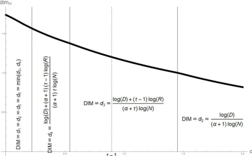
Now, we introduce the 6 different quantities, depending on probability vectors. We call these functions dimension functions.
d1pp
´q “dimp
´, dα2pp
´, p1q “
mpα, τqhpp
´q `Mpα, τqhrpp1q p1`αqlogN , dα3pp
´, p
1, p
2q “
mpα, τqhpp
´q `Mpα, τqhpp1q ` pτ ´1qhrpp2q
pτ `αqlogN ,
dα4pp
´, p1, p2, p
`, Hq “
mpα, τqhpp
´q `Mpα, τqhpp
1q ` pτ´1qhrpp
2q `αpτ ´1qhrpp
`q `αp1´1{τqH
τp1`αqlogN ,
dα5pp
´, p1, p2, p
`, Hq “
mpα, τqhpp
´q `Mpα, τqhpp1q ` pτ´1qhpp2q ` pτ `αqpτ ´1qhrpp
`q `αp1´1{τqH
τpτ `αqlogN ,
d6pp
`q “dimp
`, and let
Dαpp
´, p1, p2, p
`, hq “min
! d1pp
´q, dα2pp
´, p1q, dα3pp
´, p1, p2q, dα4pp
´, p1, p2, p
`, hq, dα5pp
´, p1, p2, p
`, hq, d6pp
`q )
. Theorem 1.1. Let xn be an arbitrary sequence of points on Λ and let f :N ÞÑ N be an arbitrary
function such that limnÑ8fpnq
n “αą0. Then
dimHtyPΛ :Tny PPfpnqpxnq infinitely oftenu “ max
p´,p
1,p
2,p
`PΥ4Dαpp
´, p1, p2, p
`,0q.
Let us denote the geometric balls on R2 centered atxand with radius r by Bpx, rq.
Theorem 1.2. Let µbe an ergodic,T-invariant measure such thatsuppµ“Λ. Letxn be a sequence of identically distributed random variables (not necessarily independent) with distribution µ and let r :NÞÑR` be an arbitrary function such thatlimnÑ8´logrpnq
nlogN “αą0. Then dimHty PΛ :TnyPBpxn, rpnqq infinitely oftenu “ max
p´,p
1,p
2,p
`PΥ4Dαpp
´, p1, p2, p
`, Hq, where H“ş
logTtN xu`1dµpx, yq.
For the heuristic explanation of the result we refer the reader to Section 3.
2. Symbolic dynamics
Let us denote by Σ the space of all infinite length words formed of symbols in Q, i.e. Σ “ QN. Let Σ˚ denote the set of finite length words, i.e Σ˚ “ Ť8
n“0Qn. Usually, we denote the elements of Σ by i,j and we denote the elements of Σ˚ by ı, ,~. For an i “ ppa1, b1q,pa2, b2q, . . .q P Σ and němě1 integer, leti|nm “ ppam, bmq, . . . ,pan, bnqq. ForıPΣ˚ andiPΣ (orPΣ˚), letıi(orı) be the concatenation of the words. We use the convention throughout the paper that for a nonnegative number pRN,ip :“itpu, wheret.udenotes the lower integer part.
For ı“ ppa1, b1q, . . . ,pan, bnqq PΣ˚, let
Cpıq “ j“ ppa11, b11q,pa12, b12q, . . .q:a1k“ak and b1k“bk fork“1, . . . , n( .
Moreover, denote Bpıq the approximate square that containsı “ ppa1, b1q, . . . ,pan, bnqq and has size N´|ı|. That is,
Bpıq “ ď
b1
tn τu`1PPa
tn τu`1
¨ ¨ ¨ ď
b1nPPan
Cpı|n{τ1 ppatn
τu`1, b1tn
τu`1q, . . . ,pan, b1nqqq.
Denote the cylinder of length ncontaining i“ ppa1, b1q,pa2, b2q, . . .q PΣ byCnpiq, i.e.
Cnpiq “Cpi|n1q andBnpiq “Bpi|n1q.
For any ı“ ppa1, b1q, . . . ,pan, bnqq PΣ˚, let
Fı“Fpa1,b1q˝ ¨ ¨ ¨ ˝Fpan,bnq. Let us define the natural projection from Σ to Λ by π. That is,
πpiq “ lim
nÑ8Fi|n
1p0,0q.
Let us denote the left-shift operator on Σ by σ. It is easy to see thatσ and T are conjugated on Λ, i.e.
π˝σ“T ˝π. (2.1)
Let f :NÞÑN be a function such that
nÑ8lim fpnq
n “α ą0. (2.2)
Lettjnube a sequence in Σ and let ΓCpf,tjnuq,ΓBpf,tjnuqbe the set of points which hit the shrinking targets tCfpnqpjnqu andtBfpnqpjnquinfinitely often. That is,
ΓCpf,tjnuq “ tiPΣ :σniPCfpnqpjnq i.o.u and ΓBpf,tjnuq “ tiPΣ :σniPBfpnqpjnq i.o.u.
In other words,
ΓCpf,tjnuq “
8
č
K“1 8
ď
k“K
σ´kpCfpkqpjkqqand ΓBpf,tjnuq “
8
č
K“1 8
ď
k“K
σ´kpBfpkqpjkqq. (2.3) For a visualisation of σ´nCfpnqpjnq,σ´nBfpnqpjnq, see Figure 1.
Theorem 2.1. Let tjnu be an arbitrary sequence in Σ, and let f :N ÞÑ N be a function such that limnÑ8fpnqn “αą0. Then
dimHπΓCpf,tjnuq “ max
p´,p
1,p
2,p
`PΥ4Dαpp
´, p1, p2, p
`,0q. (2.4)
Figure 1. Symbolic representation of holes atnth iterations defined by cylinders and balls. That is, the sets σ´nCfpnqpjnq and σ´nBfpnqpjnq.
Theorem 2.2. Let f : N ÞÑ N be a function such that limnÑ8fpnq
n “ α ą 0 and let tjn “ ppapnq1 , bpnq1 q,papnq2 , bpnq2 q, . . .qube a sequence inΣsuch thatlimnÑ8fpnqp1´1{τq1
řfpnq
k“fpnq{τlogT
apnqk “H.
Then
dimHπΓBpf,jkq “ max
p´,p
1,p
2,p
`PΥ4Dαpp
´, p
1, p
2, p
`, Hq. (2.5)
3. Heuristics
The statements of our results might on the first glance look a bit strange and complicated, but they have a simple geometric meaning.
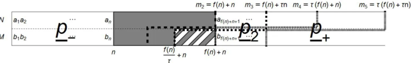
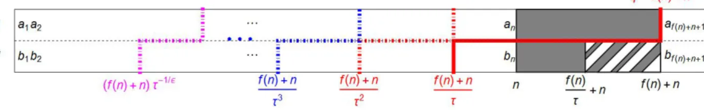
Fix some n ą 0 and consider the set Γn of points that hit the target at time n. In symbolic description, Γnconsists of points that have prescribed symbols on positionsai, i“n`1, . . . , n`fpnq and bj, j “n`1, . . . , n`τ´1fpnq (in the ball case) or on positions ai, i“n`1, . . . , n`fpnq and bj, j “n`1, . . . , n`fpnq(in the cylinder case). Letp´, p1, p2, p`be some fixed probabilistic vectors on Q.
We will define a probabilistic measure µn“µnpp´, p1, p2, p`qthe following way. We will demand thatpai, biqis independent frompaj, bjqfor alli‰j, and that the distribution ofpai, biqis given byp´
for iďminpn, τ´1pn`fpnqqq, by p1 forτ´1pn`fpnqq ăiďn, by p2 forn`fpnq ăiďτ n`fpnq, and by p` for i ą τ n`fpnq. If we are in the ball case then we still have to describe bi for n`τ´1fpnq ă i ď n`fpnq, at those position we have already prescribed the value of ai and we distribute bi choosing each of available values ofbi PPai with the uniform probability 1{Tai.
Given m, we define the local dimension ofµn at a pointj at a scale N´m by dmpµn,jq “ logµnpBmpjqq
´mlogN .
Then, everywhere except at aµn-small set of points, we will have that the local dimensions ofµn at scales N´mi corresponds to the dimensions values di as follows:
m1 !n m2 “n`fpnq m3“τ n`fpnq m4 “τpn`fpnqq m5 “τpτ n`fpnqq m6 "n`fpnq d1pp´q dα2pp´, p1q dα3pp´, p1, p2q dα4pp´, p1, p2, p`q dα5pp´, p1, p2, p`q d6pp`q For a visual representation of the approximate squares at level mi, see Figure 2 and Figure 3.
Moreover, one can check that, again everywhere except at a µn-small set of points, the local minima of dmpµn,jq happen at (some of) the scalesm1, . . . , m6. That is, formiămămi`1 we have
Figure 2. The representations of balls at scale mi and the probability measure µn
in the case αěτ´1.
Figure 3. The representations of balls at scale mi and the probability measure µn
in the case αăτ´1.
dmpµn,jq ąminpdmipµn,jq, dmi`1pµn,jqq ´εpnq, where εpnqis small for nlarge.
The rest of the paper is divided as follows. The following section is devoted to prove several lemmas, used heavily later in the proofs of lower and upper bounds. In Section 4.1, we define a class of measures (piecewise Bernoulli measures) which are a generalization of the measure µn defined above.
In particular, a piecewise Bernoulli measure is the distribution of a sequence of independent finite valued random variables, chosen in a piecewise constant way. That is, we consider a sequence of intervals pSk´1, Sks P N and a sequence of finite valued random variables Xk, and at all the positions iP pSk´1, Skswe use the random variable Xk. We show that the local dimension of such measures (more precisely, of their projections from the symbolic space, where they are defined, to the Bedford-McMullen carpet) can be calculated by considering only the scales correspoding to the positions Sk (Lemma 4.3), which lets us to write explicite formulas (Lemma 4.2). Those measures will be eventually used in Section 5, to obtain the lower bounds, since the projection of a well-chosen piecewise Bernoulli measure gives full measure to the shrinking target set.
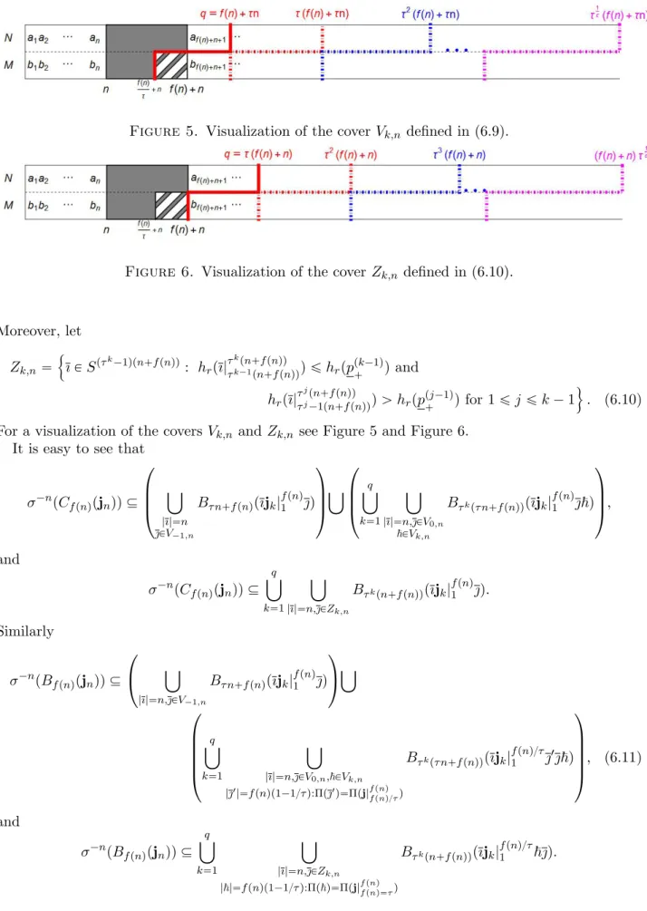
In Section 4.2, we will present the basic properties of entropy and row entropy (Lemma 4.5), and give some counting arguments (Lemma 4.6, Lemma 4.7 and Lemma 4.8), which will be useful during the proof of upper bound. Moreover, Lemma 4.5 is also applied to simplify significantly the statements of our results. Namely, it allows us in Section 4.3 to work with a restricted family of probabilities (Lemma 4.9) and Lemma 4.10), and to show some relations between the values of functions dαi, where the minimum is achieved (Lemma 4.11). The construction of the cover depends on, which function dαi achieve the minimum value in Dα at the maximum. The case of dα6 “Dα is the most difficult and in order to be able to handle this case, Lemma 4.11 plays a key role in the argument (see Lemma 6.5 and Lemma 6.11).
In Section 5, we will prove the lower bound estimation for the dimension of the shrinking target set. With a proper choice of tniu, we will construct a piecewise Bernoulli measure supported on the set of points that hit the targets at times tniu in such a way that around each scale N´ni this measure will be similar to µni. In Section 6, we will prove the upper bound estimation. Idea of
proof: for any nwe will construct a cover for all the points hitting the target at time n. Again, the construction of this cover will be closely related to the measure µn, though this relation might be difficult to explain right now. We finish the paper with the examples section.
4. Entropy and piecewise Bernoulli measures
4.1. Piecewise Bernoulli measures. We definethe piecewise Bernoulli measures on Σ as follows.
Let ppkq be an arbitrary sequence in Υ and let mk be a sequence of positive integers. Let us denote řk
q“1mq by Sk with the concept S0 “0. Then we call µpiecewise Bernoulli if µ“
8
ź
`
η`“1, whereη` “ppkq if`P pSk´1, Sks.
Lemma 4.1. Let ppkq be a sequence of probability vectors in Υ and let mk be a sequence of integers such that
8
ÿ
k“1
m´1k ă 8. (4.1)
Let µ be the piecewise Bernoulli measure corresponding to the sequences ppkq and mk. Then there exists a setΩwithµpΩq “1such that for every sufficiently smallεą0and for everyi“ pi1, i2, . . .q P Ω there exist K “Kpε,iq such that for every kěK and every εmk´1 ămďmk
ˇ ˇ ˇ ˇ ˇ
7t`“1`řk´1
q“1mq, . . . , m`řk´1
q“1mq :i` “ju
m ´ppkqj
ˇ ˇ ˇ ˇ ˇ
ăε and ˇ
ˇ ˇ ˇ ˇ
7t`“řk
q“1mq´m`1, . . . ,řk
q“1mq:i` “ju
m ´ppkqj
ˇ ˇ ˇ ˇ ˇ
ăε.
Proof. We prove only the first inequality, the proof of the second one is similar.
Let us recall here Chebyshev’s inequality. Let X1, X2, . . . be independent, uniformly bounded random variables. Then for every εą0
P
˜ˇ ˇ ˇ ˇ ˇ
n
ÿ
i“1
Xi´
n
ÿ
i“1
EpXiq ˇ ˇ ˇ ˇ ˇ
ąnε
¸ ď C
n2 for allně1, (4.2)
where C is some constant depending on the uniform bound and εą0.
Let us fix εą0. Let ∆m,k be the set of iPΣ such that ˇ
ˇ ˇ ˇ ˇ
7t`“1`řk´1
q“1mq, . . . , m`řk´1
q“1mq:i` “ju
m ´ppkqj
ˇ ˇ ˇ ˇ ˇ
ąε.
Then by (4.2),
µp∆m,kq ă C m2. Hence,
µ
˜ m
k
ď
m“εmk´1
∆m,k
¸ ď
mk
ÿ
m“εmk´1
C
m2 ď Cp1´εq εmk´1
. Since the series ř8
k“1m´1k is summable, by Borel-Cantelli Lemma the assertion follows.
Let iPΣ andqě1. Let k, `be integers such that Sk´1 ďq ăSk and τ S`´1 ďq ăτ S`, then µpBqpiqq “
`´1
ź
n“1 Sn
ź
r“Sn´1
ppnqa
r,br ¨
q{τ
ź
r“S`´1
pp`qa
r,br¨
S`
ź
r“q{τ
pp`qar ¨
k´1
ź
n“``1 Sn
ź
r“Sn´1
ppnqar ¨
q
ź
r“Sk´1
ppkqar . (4.3) Lemma 4.2. Let C ĂΥo be compact set and let tppkqu8k“1 be a sequence of prob. vectors such that ppkqPC for all kě1. Moreover, tmku8k“1 be a sequence of integers such that (4.1) hold. If µ is the piecewise Bernoulli measure corresponding to mk and ppkq then forµ-a.e. i
lim inf
kÑ8
logµpBSkpiqq
´SklogN “ lim inf
kÑ8
ř`pkq´1
n“1 mnhpppnqq ` pSk{τ ´S`pkq´1qhppp`qq ` pS`pkq´Sk{τqhrppp`qq `řk
n“``1mnhrpppnqq
SklogN ,
(4.4) where `pkq is the unique integer such that τ S`pkq´1 ďSkăτ S`pkq, and
lim inf
`Ñ8
logµpBτ S`piqq
´τ S`logN “lim inf
`Ñ8
ř`
n“Kmnhpppnqq `řkp`q´1
n“``1mnhrpppnqq ` pτ S`´Skp`q´1qhrpppkqq
τ S`logN ,
(4.5) where kp`q is the unique integer such that Skp`q´1 ďτ S` ăSkp`q.
Proof. We prove only equation (4.4), the proof of (4.5) is similar and even simpler.
By (4.3),
µpBSkpiqq “
`pkq´1
ź
n“1 Sn
ź
r“Sn´1
ppnqa
r,br¨
Sk{τ
ź
r“S`pkq´1
pp`qa
r,br ¨
S`pkq
ź
r“Sk{τ
pp`qar ¨
k
ź
n“`pkq`1 Sn
ź
r“Sn´1
ppnqar .
Letεą0 be arbitrary, but fixed. LetK “Kpε,iq ą0 be the constant defined in Lemma 4.1 and let us assume that`pkq ąK`1. Thus,
logµpBSkpiqq
´SklogN ě ř`pkq´1
n“K mnhpppnqq `řk
n“`pkq`1mnhrpppnqq ´řSk{τ
r“S`pkq´1logpp`qa
r,br ´řS`pkq
r“Sk{τlogpp`qar
SklogN ´C1ε (4.6)
and
logµpBSkpiqq
´SklogN ď ř`pkq´1
n“K mnhpppnqq `řk
n“`pkq`1mnhrpppnqq ´řSk{τ
r“S`pkq´1logpp`qa
r,br ´řS`pkq
r“Sk{τlogpp`qar
SklogN `
` SKPˆ
SklogN `C1ε, (4.7) with some constant C1ą0 and ˆP “ ´minpPCmina,blogpa,b. There are three possible cases,
‚ ifτ S`pkq´1 ďSkďτ S`pkq´1`ετ m`pkq´1 then by Lemma 4.1
´
Sk{τ
ÿ
r“S`pkq´1
logpp`qa
r,br ´
S`pkq
ÿ
r“Sk{τ
logpp`qar ďεm`pkq´1Pˆ` pS`pkq´Sk{τqhrppp`qq `m`εď
pSk{τ ´S`pkq´1qhppp`qq ` pS`pkq´Sk{τqhrppp`qq ` p1`PˆqSkε and
´
Sk{τ
ÿ
r“S`pkq´1
logpp`qa
r,br ´
S`pkq
ÿ
r“Sk{τ
logpp`qar ě pS`pkq´Sk{τqhrppp`qq ´m`εě
pSk{τ ´S`pkq´1qhppp`qq ` pS`pkq´Sk{τqhrppp`qq ´εSkmax
pPC hppq.
‚ Similarly, if τ S`pkq´ετ m`pkq´1 ďSk ďτ S`pkq pSk{τ ´S`pkq´1qhppp`qq ` pS`pkq´Sk{τqhrppp`qq ´εSkmax
pPC hrppq ď
´
Sk{τ
ÿ
r“S`pkq´1
logpp`qa
r,br ´
S`pkq
ÿ
r“Sk{τ
logpp`qar ď
pSk{τ´S`pkq´1qhppp`qq ` pS`pkq´Sk{τqhrppp`qq ` p1`PˆqSkε, (4.8)
‚ and if τ S`pkq´1`ετ m`pkq´1ăSkăτ S`pkq´ετ m`pkq´1 then ˇ
ˇ ˇ ˇ ˇ ˇ
pSk{τ ´S`pkq´1qhppp`qq ` pS`pkq´Sk{τqhrppp`qq ´
¨
˝´
Sk{τ
ÿ
r“S`pkq´1
logpp`qa
r,br ´
S`pkq
ÿ
r“Sk{τ
logpp`qar
˛
‚ ˇ ˇ ˇ ˇ ˇ ˇ
ď2εSk. Equation (4.4) follows from the fact that the choice of εwas arbitrary.
Lemma 4.3. Let C ĂΥo be compact set and let tppkqu8k“1 be a sequence of prob. vectors such that ppkqPC for all kě1. Moreover, tmku8k“1 be a sequence of integers such that (4.1) hold. If µ is the piecewise Bernoulli measure corresponding to mk and ppkq then forµ-a.e. i
lim inf
qÑ8
logµpBqpiqq
´qlogN “min
"
lim inf
kÑ8
logµpBSkpiqq
´SklogN ,lim inf
`Ñ8
logµpBτ S`piqq
´τ S`logN
* .
Proof. Let εą0 be arbitrary small but fixed. Let i PΩ and let K “Kpi, εq, where the set Ω and the constant K “ Kpε,iq defined in Lemma 4.1. Let k, ` be integers such thatSk´1 ďq ă Sk and τ S`´1ďq ăτ S`. We may assume that `ąK`1.
If qP pSk´1, Sk´1`εmk´1q then logµpBqpiqq
´qlogN ě logµpBSk´1piqq
´pSk´1`εmk´1qlogN ě 1 1`ε
logµpBSk´1piqq
´Sk´1logN . (4.9)
Similarly, if q P pτ S`´1, τ S`´1`ετ m`´1q then logµpBqpiqq
´qlogN ě 1 1`ε
logµpBτ S`´1piqq
´τ S`´1logN . (4.10)
So without loss of generality, we may assume that
Sk´1`εmk´1ďq ďSk and τ S`´1`ετ m`´1 ďq ďτ S`.
By Lemma 4.1 and (4.3), logµpBqpiqq
´qlogN ě ř`´1
n“Kmnhpppnqq ` pq{τ ´S`´1qhppp`qq ´řS`
r“q{τlogpp`qar `řk´1
n“``1mnhrpppnqq ` pq´Sk´1qhrpppkqq
qlogN ´C1ε,
where C1 depends only on ε ą 0 and the compact set C but independent of q. If q P pτ S` ´ ετ m`´1, τ S`q then the right hand side is greater than or equal to
logµpBqpiqq
´qlogN ě ř`
n“Kmnhpppnqq `řk´1
n“``1mnhrpppnqq ` pτ S`´Sk´1qhrpppkqq
τ S`logN ´C2ε, (4.11)
where C2ěC1 but depend only on εą0 and the compact set C.
On the other hand, if q P pτ S`´1`ετ m`´1, τ S`´ετ m`´1q then by Lemma 4.1 logµpBqpiqq
´qlogN ě ř`´1
n“Kmnhpppnqq ` pq{τ ´S`´1qhppp`qq ` pS`´q{τqhrppp`qq `řk´1
n“``1mnhrpppnqq ` pq´Sk´1qhrpppkqq
qlogN ´Cε.
Clearly, the right hand side of the inequality is either strictly increasing or strictly decreasing in q, thus
logµpBqpiqq
´qlogN ě min
q“Sk´1,τ S`´1,Sk,τ S`
# ř`´1
n“Kmnhpppnqq ` pq{τ ´S`´1qhppp`qq qlogN
`pS`´q{τqhrppp`qq `řk´1
n“``1mnhrpppnqq ` pq´Sk´1qhrpppkqq qlogN
+
´Cε. (4.12) Hence, the statement of the lemma follows by Lemma 4.2, (4.9),(4.10),(4.11), (4.12) and the fact
that the choice of εąwas arbitrary.
4.2. Notes on entropy and coverings. Let pD be the unique measure with maximal entropy, let pRbe the measure with maximal entropy among the measures with maximal row-entropy, and letpd be the measure with maximal dimension. That is,
pD “ ˆ1
D
˙
pa,bqPQ
, pR“ ˆ 1
TaR
˙
pa,bqPQ
, pd“
¨
˝ T
1 τ´1 a
ř
a1PST
1 τ
a1
˛
‚
pa,bqPQ
. (4.13)
The first two formulas are obvious. The proof for the third one can be found in [6, Theorem 4.5] or alternatively [23, Theorem on p. 1].
Lemma 4.4. The functionspÞÑhppq,pÞÑhrppq, pÞÑdimppq are continuous and concave on Υ.
Proof. Proof is straightforward.
Given 0ďzďlogR let
ψpzq “maxthppq:hrppq “zu, and for 0ďzďlogD
ϕpzq “maxthrppq:hppq “zu.
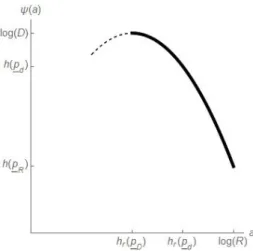
Lemma 4.5. The functions aÞÑψpaq, aÞÑϕpaq, aÞÑ ψpaq`pτ´1qa
logM and aÞÑ a`pτ´1qϕpaq
logM are concave on their domains. Moreover, hrppDq ďhrppdq ďhrppRq “logR andhppRq ďhppdq ďhppDq “logD and equalities hold if and only if Ta takes only one value for all aPS.
Proof. First, we prove the concavity of ψ. It is easy to see that for any p P Υ, hpp1q ě hppq and hrpp1q “hrppq, where
p1a,b“ ř
bpa,b
Ta “ pa Ta. Hence,
ψpzq “z`maxtÿ
aPS
palogTa:´ ÿ
aPS
palogpa“zu.
However,
maxtÿ
aPS
palogTa:´ ÿ
aPS
palogpa“zu “maxtÿ
aPS
palogTa:´ ÿ
aPS
palogpaězu.
Indeed, the ď direction is trivial. Let 71 “ 7ta P S : Ta “ mina1PSTa1u and 72 “ 7ta P S : Ta “ maxa1PSTa1u. IftpauaPS is a maximizing vector such that´ř
aPSpalogpaąz then by choosing p1a“
$
’&
’%
pa´δ{71, ifas.t. Ta“mina1PSTa1; pa`δ{72, ifas.t. Ta“maxa1PSTa1; pa, otherwise
we have ř
aPSpalogTa ă ř
aPSp1alogTa and ´ř
aPSp1alogp1a ą z for sufficiently small choice of δ, which contradicts to the assumption that tpauaPS is a maximizing vector.
Therefore,
qψpz1q ` p1´qqψpz2q “ qz1` p1´qqz2`maxtÿ
aPS
qpa` p1´qqp1alogTa:´ÿ
aPS
palogpaěz1, ´ÿ
aPS
p1alogp1aěz2u ď qz1`p1´qqz2`maxtÿ
aPS
qpa`p1´qqp1alogTa:´ ÿ
aPS
pqpa`p1´qqp1aqlogpqpa`p1´qqp1aq ěqz1`p1´qqz2u “ ψpqz1` p1´qqz2q.
The concavity ofϕ follows by the fact thatϕpψpzqq “z forzP rhrpp
Dq,logRs.
The proof of the second statement of the lemma follows from simple algebraic manipulations.
For the graph of the function ψ on rhrppDq,logRs, see Figure 4.
Let us denote the symbolic space formed by only the row symbols by Ξ“SNand the set of finite length words by Ξ˚ “Ť8
n“0Sn. Let Π be the natural correspondence function between Σ and Ξ (and between Σ˚ and Ξ˚ respectively). That is, fori “ ppa1, b1q,pa2, b2q, . . .q PΣ let Πpiq “ pa1, a2, . . .q (and for ı“ ppa1, b1q, . . . ,pan, bnqq PΣ˚ let Πpıq “ pa1, . . . , anq).
For a finite wordıPΣ˚ and forPΞ˚let us define the entropy ofıand row-entropy ofas follows.
Let us denote the frequency of a symbol pa, bq and a row-symbol ainı and by υa,bpıq “ 7tk“1, . . . ,|ı|:pak, bkq “ pa, bqu
|ı| andυapq “ 7tk“1, . . . ,||:ak“au
|| .
We can also define the frequency of rows for finite words ıPΣ˚ in the natural way, υapıq:“υapΠpıqq “ ÿ
bPPa
υa,bpıq.
Figure 4. The graph of the function ψon rhrppDq,logRs.
And let for ıPΣ˚ and PΞ˚ hpıq “ ´ ÿ
pa,bqPQ
υa,bpıqlogυa,bpıq, hrpıq “ ´ÿ
aPS
υapıqlogυapıq and hrpq “ ´ÿ
aPS
υapqlogυapq.
Lemma 4.6. For every εą0 there exists N ě1 such that for all něN and every hďlogD and hrďlogR
7 tıPQn:hpıq ďhu ďenph`εq and
7 tPSn:hrpq ďhru ďenphr`εq.
Proof. We prove only the first inequality, the proof of the second one is analogous.
Let W “ tpPΥ :hppq ďhu. Then tıPQn:hpıq ďhu “ ď
pqpa,bqqpa,bqPQPND ř
pa,bqPQ
qpa,bq“n
´ ř
pa,bqPQ qpa,bq
n logqpa,bqn ďh
ıPQn:va,bpıqn“qpa,bq forpa, bq PQ( .
For any qpa,bqPNwith ř
pa,bqPQqpa,bq“n,
7 ıPQn: va,bpıqn“qpa,bq forpa, bq PQ(
“ n!
ś
pa,bqPQ
qpa,bq!. By using Stirling’s formula, there exists Cą0 such that for everykě1
C´1kk ek
?2πk ďk!ďCkk ek
?2πk.
Thus, for anyqpa,bq PNwithř
pa,bqPQqpa,bq“nand with´ ř
pa,bqPQ qpa,bq
n logqpa,bqn ďh n!
ś
pa,bqPQ
qpa,bq!“ n!
ś
pa,bqPQ qpa,bqě1
qpa,bq!ďCD`1? ne´n
ř
pa,bqPQ qpa,bq
n logqpa,bqn
ďCD`1? nenh.
On the other hand, 7tpqpa,bqqpa,bqPQ PND : ř
pa,bqPQ
qpa,bq “nu ď`n`D`1
D
˘. Hence, for every εą0 one can choose N ą1 such that for everyněN
tıPQn:hpıq ďhu ď
ˆn`D`1 D
˙
CD`1?
nenh ďenph`εq.
Lemma 4.7. For every z P rhrpp
Dq,logRs and for every ε ą 0 there exists N ą 0 such that for every nąN
7tıPQn:hrpıq ězu ďenpψpzq`εq.
Moreover, For every x P rhppRq,logDs and for every εą0 there exists N1 ą0 such that for every nąN1
7ΠtıPQn:hpıq ěxu ďenpϕpxq`εq.
Proof. By Lemma 4.5, ψpzq is monotone decreasing on the intervalrhrppDq,logRs. So, if hrpıq ěz then hpıq ďψphrpıqq ďψpzq. Thus, the statement follows by Lemma 4.6.
Lemma 4.8. LetVn be a set of finite length words with lengthn. Denote the number of approximate squares with side length N´n required to cover V “Ť
ıPVnBnpıq by Vn1. Then Vn1 ď 7tPQn{τ :“ı|n{τ1 u ¨ 7t1 PSnp1´1{τq : Πpı|nn{τ`1q “1u.
The proof is straightforward.
4.3. Properties of the dimension functions. Let Υψ :“
!
pPΥ :ψphrppqq “hppq &hrppq ěhrppDq )
, and let
Θ :“
! pp´, p
1, p
2, p
`q P pΥψq4 :hrpp
´q P rhrpp
Dq, hrpp
dqs, hrpp
1q P rhrpp
´q,logRs and hrpp
`q P rhrppdq,logRs )
, where p
R, p
d andp
D are defined in (4.13).
Lemma 4.9. For any hě0,
p max
´,p
1,p
2,p
`PΥDαpp
´, p
1, p
2, p
`, hq “ max
pp´,p
1,p
2,p
`qPΘDαpp
´, p
1, p
2, p
`, hq Proof. It is easy to see that Dαpp
´, p
1, p
2, p
`, hq is monotone increasing in hpp
iq and hrpp
iq for i “ ´,1,2,`. Thus, for fixed hrppiq the value of Dα can be increased by replacing hppiq with ψphrppiqq.
On the other hand, since ψ is continuous and concave with maxima athrppDq, if hrppDq ěhrppiq for some i“ ´,1,2,` then the value ofDα can be increased by replacing hrppiq with hrppDq, and replacing hpp
iq “ψphrpp
iqq with logD“hpp
Dq. Thus, we’ve shown that
p max
´,p
1,p
2,p
`PΥDαpp
´, p
1, p
2, p
`, hq “ max
pp´,p
1,p
2,p
`qPpΥψq4
Dαpp
´, p
1, p
2, p
`, hq.
Now, let pp
´, p1, p2, p
`q P pΥψq4 be arbitrary. Since the function a ÞÑ ψpaq`pτ´1qa
logM is a concave function with maxima ata“hrpp
dqandaÞÑψpaqis strictly decreasing onrhrpp
Dq,logRs, ifhrpp
´q ą hrppdqthen by choosingp1“ p1´εqp
´`εpd, we get thatdipp1, p1, p2, p
`q ądipp
´, p1, p2, p
`qfor every i“1, . . . ,5. Thus,Dαpp1, p
1, p
2, p
`q ěDαpp
´, p
1, p
2, p
`q and we may assume thathrpp
´q ďhrpp
dq.