Effect Size Calculation in Power Estimation for the Chi-square Test of Preliminary Data in Different Studies
Anna Laszlo1, Agnes Feher2, Anna Juhasz3, Tibor Nyari4, Krisztina Boda5, Jozsef Csicsman6, Ferenc Bari7
1,4,5,7 Department of Medical Physics and Informatics, Faculty of Medicine, University of Szeged, Szeged, Hungary
2,3 Department of Psychiatry, Faculty of Medicine, University of Szeged, Szeged, Hungary
6 Institute of Mathematics, Faculty of Natural Sciences, Budapest University of Technology and Economics, Budapest, Hungary
1laszlo.anna@med.u-szeged.hu; 2feher.agnes@med.u-szeged.hu; 3juhasz.anna@med.u-szeged.hu;
4nyari.tibor@med.u-szeged.hu; 5boda.krisztina@med.u-szeged.hu; 6csicsman@math.bme.hu; 7bari.ferenc@med.u- szeged.hu
Abstract
The validity of statistical analyses applied to identify different factors in many fields depends upon the use of appropriate sample sizes, the lack of which reduces the power of the findings. However, the number of cases collected for data analysis in medical studies is generally limited, for medical, financial and other experimental reasons, and statistical tests are often carried out without power and sample size estimation. Power analysis involves several parameters, the most important of which, the effect size, reflects the degree of the effect expected to be found in the study. An easy-to-use MS Excel calculator has been constructed to determine the effect size for chi-square tests based on 2×2, 2×3 and 2×4 contingency tables, and compared the results obtained with this calculator with those given by GPower, R and, for a 2×2 table, SAS software to demonstrate the practical use of this calculation tool in three studies involving various data.
Keywords
Frequency Data; Contingency Table; Preliminary Study; Effect Size; Statistical Power Estimation; GPOWER; R; SAS
Introduction
The independence of two quantitative grouping variables can be investigated by creating a contingency table [Pearson, 1904]. p-values for the comparison of these categorical variables can be calculated using chi- square tests, the statistical method most frequently used to detect differences between proportions [Agresti, 2002], supported by most statistical software.
Power calculation has recently received increasing attention in statistical analysis as an essential tool to determine an appropriate sample size, or to obtain a
power which indicates the reliability of the statistical test based on preliminary data [Cohen, 1988; Gordon et al., 2002]. Power is considered highly important in experimental design, where it is applied before data collection, but it is itself also based on preliminary information (which can be obtained from a pilot study) [Osmena, 2010].
Most statistical tests have their specific calculation methods for power estimation; in this paper, we focus on power calculations for the chi-square test, which are well known [Cohen, 1988]. To determine the power of a statistical test, a few input parameters have to be set, the most crucial of them being the effect size.
The determination of effect size is a medical problem:
which is generally given by a physician or researcher on the basis of earlier experience. When the examined field is a new one and there are no previous results to find an appropriate effect size, it can be determined from new data, but only with the use of a preliminary set.
The power of a statistical test is the probability of correctly finding a difference (rejecting the null hypothesis) between the investigated variables with the statistical test.
There are several arguments that a post-hoc power calculation is meaningless [Hoenig et al., 2001; Lenth, 2001]. During research in which power is calculated, it is mostly done after the experiment has been finished, i.e. retrospectively, which is as much a mistake as it is useful in the design phase. Hoenig et al. showed why there is no reason to run a power analysis when a result was significant [Hoenig et al., 2001]. Researchers
have to handle this topic with foresight.
Power analysis is available in several free software packages (e.g. R or GPower). A comparison of power analysis for the chi-square test in the R and SAS systems revealed both advantages and disadvantages of the possibilities in the methods applied by the two programs [Osmena, 2010]. However, these packages utilize effect size as an input parameter. If it is not given by an expert, but a preliminary data set is available, calculation of the effect size is possible.
To simplify effect size calculation from a contingency table, an MS Excel calculator has been constructed (Appendix II), and compared with calculations in R (for a 2×2 contingency table, an R script is given in Appendix III), in GPower software, and for 2×2 contingency tables in SAS.
Other effect size calculators for the chi-square test are freely available via the internet (including MS Excel- based ones) [DeFife, 2009; Ellis, 2009; Wilson, 2001], but these mostly work with the formula based on the chi-square test statistic and the total number of cases, rather than frequency data in a contingency table, which we applied [Cohen, 1988]. These calculators are mainly created for 2×2 contingency tables, but we have extended the dimensions to 2×3 and 2×4 tables.
Aim
Our primary aim was to evaluate the effect size for power estimation for chi-square tests as a demonstration of the analysis in different studies using an MS Excel-based calculator based on pilot studies. A further goal was to run power calculations on additional experimental data, using the calculated effect size. The easy-to-use MS Excel calculator was compared with other software (R, GPower and SAS;
see the section Programs Used in the Methods) in order to prove our results.
Methods Definitions
The null hypothesis of the chi-square test for independence can be tested by the following formula:
𝜒𝜒2= �(𝑂𝑂𝑖𝑖− 𝐸𝐸𝑖𝑖)2 𝐸𝐸𝑖𝑖
𝑚𝑚
where: 𝑖𝑖=1
Oi = observed frequency
Ei = expected frequency, asserted by the null
hypothesis
m = number of cells [Osmena, 2010].
“The distribution of the χ2-statistic follows a central chi-square distribution when the null hypothesis is true. When the null hypothesis is false it follows a noncentral chi-square distribution with the noncentrality parameter, λ”, where λ=(effect size)2 (total sample size) [Osmena, 2010].
Therefore, the power can be defined as the probability 𝑃𝑃�𝜒𝜒2(𝑑𝑑𝑑𝑑,𝜆𝜆)≥ 𝜒𝜒1−𝛼𝛼2 (𝑑𝑑𝑑𝑑)� [Osmena, 2010].
As the chi-square test is used to check the independence between investigated categorical variables, two-sided tests are carried out during analyses.
The function pwr.chisq.test() in the pwr library of R uses the following parameters to perform power analysis:
− Effect size
− Total number of observations
− Degrees of freedom
− Level of significance
− Power
Effect size (w): This is the size of the effect that is expected to be found in the study [Osmena, 2010].
From another aspect it is a pure number which increases with the degree of discrepancy between the distribution of the alternate hypothesis and the null hypothesis (viz. the difference from the null hypothesis that we expected to detect) [Cohen, 1988], or in other words, the difference between the investigated populations which considered from the background of the specific (i.e. clinical) field. From the genetics point of view, the w is a measure of the separation of individual phenotypes based on their genotypes [Gordon et al., 2005].
In the R program, the ES.w1() and ES.w2() functions of the pwr package can be used to calculate w [Osmena, 2010].
Total number of observations (N): This is the number of all nonmissing cases in a study that compares two grouping variables (and thus the overall number of cases in the investigated contingency table).
Degrees of freedom (df): This is the number of rows in the contingency table minus 1 multiplied by the
number of columns in the contingency table minus 1 (viz. the number of cells that need to be known in the contingency table in order to calculate the others the row and column totals given).
Level of significance (α): This is also called the Type I error, which reflects the probability of a significant statistical test when there is no real difference between the compared populations (viz. the probability that the null hypothesis is true, but it is rejected: our result is false-positive).
Power (1-β): “The power of a statistical test is the probability of correctly rejecting the null hypothesis when it is false” [Osmena, 2010]. β is the probability of failing to obtain a significant difference between the investigated populations with the statistical test when there is a real difference in the background. It is also known as the Type II error rate, or the probability of a false-negative result when the null hypothesis is false, but it is failed to be rejected. In each statistical test, a lower Type II error is expected to acquire as well as a higher power (as β approaches 0, 1-β approaches 1).
Any four of these parameters determine the fifth.
Hence, when we are interested in estimation of the value of power, we set the values of w, N, df and α for our study.
Relationships between these parameters:
When w is large the 1-β is also large in the event of a fixed N, α and β. By contrast, if there is a small w, 1-β will be low and more samples are needed to detect the small w.
As α increases, β decreases, and power increases and vice versa. As α increases, N decreases, and as α decreases, N increases [Osmena, 2010].
To estimate the effect size for the chi-square test, an MS Excel-based calculator has been constructed for 2×2, 2×3 and 2×4 contingency tables, applying Cohen’s formula
𝑤𝑤 =��(𝑃𝑃1𝑖𝑖− 𝑃𝑃0𝑖𝑖)2 𝑃𝑃0𝑖𝑖
𝑚𝑚
𝑖𝑖=1
where:
P1i :“the proportion in cell i posited by the alternate hypothesis” (observed proportion of element i in the cross-classification table).
P0i: “the proportion in cell i posited by the null hypothesis” (expected proportion of element i in the
cross-classification table).
m: the number of cells in the contingency table [Cohen, 1988; Osmena, 2010].
Our MS Excel calculator was compared with the R and GPower programs. For the 2×2 contingency tables used in two studies, the power estimation was also compared with SAS, and an R script was written (Appendix III).
Without calculating the effect sizes, Cohen’s suggestion of small, medium and large w (0.1, 0.3, 0.5, respectively) can also be used, depending on how large a difference expected to find in the study [Cohen, 1988; Osmena, 2010].
The following sections present short descriptions of the three studies.
Study 1: Alzheimer’s Disease Data
Alzheimer’s disease (AD) is a neurodegenerative disorder, the most prevalent form of dementia [Selkoe, 2001], in the development of which genetic factors play an important role. Identification of AD susceptibility genes would markedly promote an understanding of the pathophysiology of the disease [Bekris et al., 2010].
An important candidate gene for AD is 24- dehydrocholesterol reductase (DHCR24), the polymorphism of which (rs600491) involves a single nucleotide change resulting in 2 alleles (C and T) and 3 genotypes (CC, CT and TT) [Lämsä et al., 2007].
Lämsä et al. investigated the DHCR24 rs600491 polymorphism as regards the risk of AD in a Finnish sample, and found that the CC, CT and TT genotype frequencies did not differ significantly between the AD and healthy control (HC) female groups
(NHCfemale=274, NADfemale=289; P(CC|HC)=0.11,
P(CC|AD)=0.11; P(CT|HC)=0.43, P(CT|AD)=0.48;
P(TT|HC)=0.46, P(TT|AD)=0.41; Fisher’s Exact test p=0.44) [Lämsä et al., 2007]. A Hungarian examination likewise revealed no significant difference in DHCR24 rs600491 genotype distribution between the AD and HC female populations (NHCfemale=139, NADfemale=201;
P(CC|HC)=0.137, P(CC|AD)=0.189; P(CT|HC)=0.525, P(CT|AD)=0.508; P(TT|HC)=0.338, P(TT|AD)=0.303;
χ2 test p=0.426) [Feher et al., 2012].
The effect size and power in both studies of females have been calculated, from which the results are compared.
Study 2: Physiotherapeutic Data
During an informatics project between September 2009 and May 2011, a system was developed by Calculus Ltd. and Polygon Informatics Ltd. to facilitate physiotherapeutic examinations on the human body with different wireless biosensors and with the use of other parameters collected on patients. This Physiosensor system connected to an SAS server, where the data collected and saved during the examinations can be analyzed via an online user interface. The first set of investigations in the project is related to knee joint straightening. During the test, 3 EMG sensors with an earthing strap (measuring the muscle activity), a goniometer (measuring the flexibility of a joint) and an event marker (determining time points) were used on specific muscles and part of the leg. The patient, in a sitting position, had to straighten their knee according to a specific protocol.
Before the measurement, personal and other health data were collected. Our analysis of the w and 1-β estimation used only gender in comparison with a grouping variable based on the birth date of the patient. This comparison by a chi-square test resulted in a nonsignificant p-value, and therefore the effect size and statistical power could be investigated.
Study 3: Anthropometric Data
Anthropometric parameters of first-year university students (Faculty of Medicine, University of Szeged, Hungary; aged around 18-19), including the hip and waist circumferences, were measured three times in 2010. Groups of averaged values of these parameters were compared with the count data in the chi-square test, and w and 1-β were then estimated.
Programs Used
GPower 3.1.5 (Heinrich-Heine-Universität, Düsseldorf, Germany), RStudio 0.97.248 (RStudio Inc., Boston, MA, USA) as a user friendly interface for running R (R Foundation for Statistical Computing, University of Auckland, New Zealand) scripts, SAS 9.2 (SAS Institute Inc., Cary, NC, USA) and IBM SPSS Statistics 20 (IBM Corp., Armonk, NY, USA) were used for statistical analyses. The MS Excel-based calculator was generated in Microsoft Office 2010 (Microsoft Hungary Ltd., Budapest, Hungary).
Results
Study 1: Alzheimer’s Disease Data
The Finnish dataset was based on a total of 563 female
patients (289 AD and 274 HC subjects; Table A1 in Appendix I), while the Hungarian DHCR24 rs600491 genotype frequency data contained overall 340 female patients (201 AD and 139 HC subjects; Table A2 in Appendix I).
With the ES.w2() R function w, and then, with the pwr.chisq.test() function, the observed power for the above two datasets were calculated. The Finnish dataset resulted in a wFinnish=0.054 with a 1-β=0.1918 among 563 cases at a 0.05 significance level. To achieve a power of 0.8 (80%), 3299 cases should be examined if the other parameters remain constant.
The Hungarian dataset resulted in wHungarian=0.071 with a 1-β=0.198 among 340 cases at a 0.05 significance level.
To achieve a power of 0.8, 1922 cases should be examined if the other parameters remain constant.
Using w from the pilot (Finnish) dataset in the power analysis of the Hungarian dataset, a power of 0.132 was obtained, which is slightly less than that calculated with w based on its own data. However all the data indicate a really low level of power.
It is obvious that with a larger w, a smaller N is sufficient to obtain the same level of power, when α and df are fixed. Here, it was expected the least to emphasize this difference in calculation. As there is no available clinically relevant w, we can use that calculated from the preliminary Finnish dataset (this is what people mostly do), as if it were the “true” effect size, but it is not. As w from the Finnish dataset is accessible, there is no need to calculate the w of the Hungarian dataset. From this example, it can be seen that w can be different in similar studies, so the clinically relevant w value would be appropriate. Thus, it is highly important to handle post-hoc calculations with foresight. Our comparisons therefore were based on calculation.
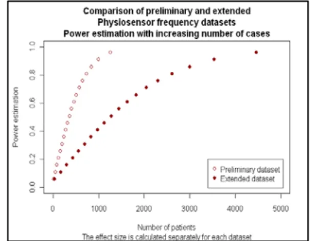
Figure 1 depicts the observed power (on the vertical axis) based on the Finnish data (empty dots) compared with the Hungarian data (filled dots) versus the number of cases (on the horizontal axis). The same Cohen formula for w and 1-β estimation for the chi- square tests [Cohen, 1988] as used in R is applied in the commonly used GPower software [Erdfelder et al., 1996]. Our MS Excel-based calculator gave the same effect size of chi-square analysis as GPower for the Hungarian data (Figure 2), but it is difficult to use GPower for the estimation of w. Figure A1 in Appendix I shows the R code with the result of the effect size and power analysis compared with Figure 2, using the same colors (magenta indicates effect size and orange
indicates the power in this paper).
As SAS calculates power only for 2×2 contingency
tables, a power analysis for the Alzheimer’s disease study failed to be performed.
FIG.1 POWER ESTIMATION (VERTICAL AXIS) FOR FINNISH AND HUNGARIAN FEMALE GENOTYPE FREQUENCY DATA WITH INCREASING TOTAL NUMBER OF FEMALES (HORIZONTAL AXIS). α=0.05, df=1, wHUNGARIAN=0.071, wFINNISH=0.054. A GREATER POWER
CAN BE ACHIEVED WITH THE HUNGARIAN THAN WITH THE FINNISH DATA BASED ON THE SAME NUMBER OF PATIENTS.
FIGURE WAS CREATED IN R.
FIG.2 COMPARISON OF OUR RESULTS WITH THE MS EXCEL CALCULATOR (LEFT-HAND PANEL) WITH THE GPOWER SOFTWARE RESULTS. IN THE EXCEL CALCULATOR, ONLY THE RED-FRAMED CONTINGENCY TABLE NEEDS TO BE COMPLETED; THE OTHER NUMBERS ARE CALCULATED AUTOMATICALLY. IN GPOWER w CAN BE CALCULATED BY USING THE PROBABILITIES FOR THE H0
(BLUE-FRAMED NUMBERS) AND H1 (GREEN-FRAMED NUMBERS) HYPOTHESES. THE RESULTING w (FROM THE RIGHT-HAND PANEL OF THE GPOWER SOFTWARE) CAN BE TRANSFERRED TO THE MAIN WINDOW (LEFT-HAND PANEL OF THE GPOWER SOFTWARE, IN THE CENTRAL PANEL OF THE FIGURE), AND POWER (ORANGE-FRAMED) CAN THAN BE DETERMINED. IT IS SEEN
THE SAME ROUNDED EFFECT SIZE VALUES ARE CALCULATED WITH EXCEL AND GPOWER (MAGENTA-FRAMED).
Study 2: Physiotherapeutic Data
The physiotherapeutic dataset was collected from the database of the Physiosensor system. As an increasing number of institutes now use the system for various medical studies (e.g. the University of Debrecen, Debrecen, Hungary, for neurological patients, or hospital in Csepel, Hungary), we had to select those cases performed in the Physiosensor laboratory (N=42).
Among the 42 observations, 34 involved the knee joint straightening protocol between February 2 and April 19 in 2011. To create a grouping variable, we differentiated the cases with respect to the median value of the birth date: the group of those born before and including 1986, and the group born in 1987 or later.
As a demonstration for power analysis, we selected the data originating from before April 1, 2011 as a pilot dataset, and then ran a chi-square test on the remaining 29 cases. The contingency table for the investigated physiotherapeutic dataset can be found in Table A3 in Appendix I.
The Pearson chi-square test resulted in a two-sided asymptotic p-value of 0.573 (the 2-sided Fisher’s Exact test gave p=0.715), showing no significant difference between the gender and birth date groups based on this dataset at a 0.05 significance level.
The data selection, variable transformation and chi- square tests were carried out in IBM SPSS Statistics 20.
w=0.105 was calculated with R, and with this value for N=29 patients and df=1 (a 2×2 contingency table) at α=0.05, 1-β=0.0872 was obtained.
For the overall period February-April 2011, the contingency table is shown in Table A4 in Appendix I.
The Pearson chi-square test resulted in a two-sided asymptotic p-value of 0.746 (the 2-sided Fisher’s Exact test gave p=1.000).
This extended study resulted in a w=0.056 (almost half of that based on the preliminary data), which at α=0.05 with df=1 leads to a power of 0.0621 for 34 observations. When the power for the extended dataset (N=34) was calculated based on the effect size of the preliminary dataset with 29 cases, a power of 0.0937 was found.
All power estimations based on physiotherapeutic datasets involving very low N resulted in almost no power for testing independence statistically from gender and birth date count data.
Figure 3 illustrates the comparison of 1-β estimations of
preliminary and extended datasets with increasing N using the separately calculated w values for the pilot study and the extended study. It is clear that, in the event of a very low N for power and sample size estimations, even a small increase in N can cause a huge difference in power estimation.
FIG. 3 COMPARISON OF POWER ESTIMATION (VERTICAL AXIS) OF PRELIMINARY (N=29) AND EXTENDED (N=34) PHYSIOTHERAPEUTIC DATASETS WITH INCREASING
NUMBERS OF PATIENTS (HORIZONTAL AXIS). w IS CALCULATED SEPARATELY FOR THE TWO STUDIES. α=0.05,
df=1, wPRELIMINARY=0.105, wEXTENDED=0.056. FIGURE WAS GENERATED IN R.
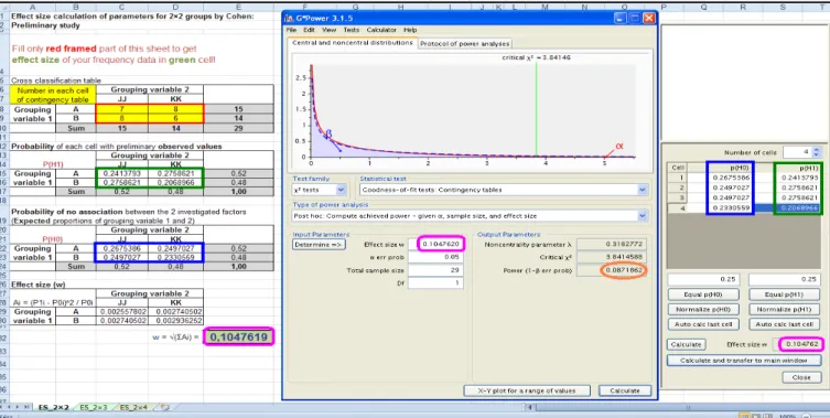
Figure 4 presents a comparison of results obtained with the MS Excel-based calculator and GPower results. The effect size and power calculation results in R was compared. The script is presented in Figure A2 in Appendix I.
The 1-β in SAS was also computed, using the w obtained with the preliminary data for estimation of the power for the extended dataset. The SAS syntax for this analysis can be found in Figure A3 in Appendix I. Figure 5 illustrates the result of the SAS syntax based on Figure A3: at N=34 SAS calculated 1-β=0.092. The same calculation in R resulted in 1-β=0.0937 (Figure A4 in Appendix I).
FIG. 5 THE RESULT OF POWER ANALYSIS IN THE SAS SYSTEM FOR GROUP PROPORTIONS OF 0.467 AND 0.571 BASED ON
PRELIMINARY PHYSIOTHERAPEUTIC DATA WITH A COMPUTED POWER FOR DIFFERENT NUMBER OF CASES.
FIG. 4 COMPARISONS OF OUR RESULTS WITH THE MS EXCEL CALCULATOR (LEFT-HAND PANEL) WITH THE GPOWER SOFTWARE RESULTS FOR PRELIMINARY PHYSIOTHERAPEUTIC DATA. IN THE EXCEL CALCULATOR, ONLY THE RED-FRAMED CONTINGENCY
TABLE NEEDS TO BE COMPLETED; THE OTHER NUMBERS ARE CALCULATED AUTOMATICALLY. IN GPOWER w CAN BE CALCULATED BY USING THE PROBABILITIES FOR THE H0 (BLUE-FRAMED NUMBERS) AND H1 (GREEN-FRAMED NUMBERS) HYPOTHESES. THE RESULTING w CAN BE TRANSFERRED (FROM THE RIGHT-HAND PANEL OF THE GPOWER SOFTWARE) TO THE
MAIN WINDOW (LEFT-HAND PANEL OF THE GPOWER SOFTWARE, IN THE CENTRAL PANEL OF THE FIGURE), AND POWER (ORANGE-FRAMED) CAN THAN BE DETERMINED. IT IS SEEN THAT THE SAME ROUNDED EFFECT SIZE VALUES ARE CALCULATED
(MAGENTA-FRAMED).
Study 3: Anthropometric Data
In the anthropometric dataset from 2010 (N=362, 181 men and 181 women) to demonstrate the w and 1-β calculation for the chi-square test, mean waist and mean hip circumference variables (measured in cm 3 times for each person) were divided into 2 categories at their median values (90 cm for the hips, and 79 cm for the waist). As the contingency table (Table A5 in Appendix I) has no cells containing an expected value less than 5, which meets the assumption of chi-square tests and can be interpreted.
Appendix I also contains results of Pearson’s chi-square tests, showing a nonsignificant difference between these two categorical variables at a 5% significance level (p=0.076) in Table A6.
Figure 6 depicts a bar chart of the frequencies (contingency table) which can be a good graphical representation of such count data. It is seen that when the waist circumference is less than its median (79 cm), slight more samples also have a lower hip circumference, and when the waist circumference is greater than its median, more samples also have a greater hip circumference (compared with
medianhip=90), a result that is probably to be expected.
FIG. 6 BAR CHART OF FREQUENCY PARTITION AMONG WAIST AND HIP CIRCUMFERENCE CATEGORIES OF THE ANTHROPOMETRIC DATASET FROM 2010. COLUMNS REFLECT NUMBERS OF 104, 80, 84 AND 94 RESPECTIVELY (SEE
TABLE A5 IN APPENDIX I).
The initial dataset was in a CSV (Comma Separated Values) format, which is usually used as the input of statistical programs. Data were then imported into IBM SPSS Statistics 20 software, and variable computation, data preparation and first comparisons
were carried out on this software. Next to investigate the w and 1-β estimation for the chi-square test, our MS Excel-based calculator was run, and the results were compared with those of GPower, R software and (as we have a 2×2 contingency table) SAS.
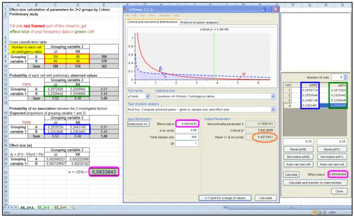
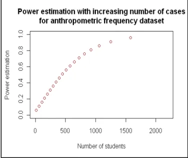
The MS Excel-based calculator and GPower gave w=0.093, which resulted in 1-β=0.427 in GPower (Figure 7). These results were also obtained with a representative dot plot (Figure 8) in R according to the script shown in Appendix III.
Plots related to the calculated power of an exact w, df, N and α can also be generated with GPower software.
A comparison of power for significance levels α=0.01 and α=0.05 is presented with increasing total sample size for anthropometric data in Figure 9. This makes it clearer that, with stronger significance levels in the power analysis (lower α), more samples must be analyzed to obtain a stronger power (closer to 1), if the other parameters remain constant.
Naturally Figures 8 and 9 for α=0.05 indicate the same result. It is expected that the results from the two software can be compared.
Conclusions
When a clinically relevant effect size as the “true”
estimate of the effect in our study is unknown, effect size can be calculated from the preliminary dataset (this can also differ from the true effect size). Without previous results, w is generally calculated on the basis of the running study, as if that w were the “truth”.
Sofwares were employed to operate the same calculation, but the interpretation of these results should be carefully considered.
In conclusion, as the usage of GPower to perform power analyses may be difficult for those without expertise in the field of statistics, an easy-to-use MS Excel calculator based on 2×2, 2×3 and 2×4 contingency tables in addition to other software is suggested. An R script for the 2×2 contingency table has been generated and such calculations have been applied to different practical studies. With such techniques, it is not difficult to calculate the effect size and power for chi- square tests and these calculations may feasibly be integrated into routine statistical analyses for researchers with biological or other backgrounds.
FIG. 7 COMPARISON OF THE RESULTS OF EFFECT SIZE CALCULATION (MAGENTA) WITH THE MS EXCEL-BASED CALCULATOR (LEFT-HAND PANEL) AND GPOWER SOFTWARE (RIGHT-HAND PANEL) BASED ON THE CONTINGENCY TABLE (SET IN THE RED-
FRAMED TABLE IN EXCEL, UPPER LEFT) OF THE ANTHROPOMETRIC DATA. PROBABILITIES CALCULATED FOR OBSERVED AND EXPECTED VALUES IN MS EXCEL CALCULATOR ARE FRAMED IN GREEN AND BLUE, RESPECTIVELY, AND ALSO SHOWN FOR GPOWER (RIGHT PANEL OF GPOWER). THE OBSERVED POWER ESTIMATION IN GPOWER SOFTWARE IS FRAMED IN ORANGE.
FIG. 8 DOT PLOT COMPARING POWER ESTIMATION (VERTICAL AXIS) WITH INCREASING NUMBER OF CASES
(HORIZONTAL AXIS) FOR ANTHROPOMETRIC DATA, DEMONSTRATING THAT TO ACHIEVE A POWER OF ABOUT 80%
ALMOST 1000 CASES SHOULD BE ANALYZED UNDER THE SAME CONDITION (df=1, α=0.05, w=0.093).
FIG. 9 COMPARISON OF POWER ESTIMATION (VERTICAL AXIS) FOR α=0.01 (RED LINE) AND α= 0.05 (BLUE LINE) WITH INCREASING TOTAL SAMPLE SIZE (HORIZONTAL AXIS) FOR ANTHROPOMETRIC DATA (df=1, w=0.0933643). THIS PLOT WAS
GENERATED BY GPOWER.
ACKNOWLEDGMENTS
We appreciate the work of Eniko Csonka for data collection from the physiotherapeutic database.
We also thank Tibor Asztalos for data collection in the anthropometric study.
This work was supported by grants TAMOP 4.2.2/A- 11/1/KONV-2012-0052, TAMOP 4.2.2/A-11/KONV-
2012-0052, TAMOP-4.2.2/B-10/1-2010-0012 and TAMOP 4.2.4.A/2-11-1-2012-0001.
REFERENCES
Agresti, A. “Categorical Data Analysis.” Second Edition, John Wiley & Sons, Inc., Hoboken, New Jersey ISBN 0- 471-36093-7, Sections 1.3, 1.5, 3.2, 3.5, 3.7. 2002.
Bekris, L.M, Yu, C.E, Bird, T.D, Tsuang, D.W. “Genetics of Alzheimer disease.” Geriatric Psychiatry and Neurology 23, 213–227. 2010.
Cohen, J. “Statistical Power Analysis for the Behavioral Sciences.” 2nd ed., Lawrence Erlbaum Associates, Inc., Hillsdale, New Jersey ISBN 0-8058-0283-5, p. 1, 216–226.
1988.
DeFife, J. Effect size calculator in MS Excel. Emory University, 2009.
Ellis, P.D. (2009), "Effect size calculators" website http://www.polyu.edu.hk/mm/effectsizefaqs/calculator/c alculator.html accessed on 01-11-2013
Erdfelder, E, Faul, F, Buchner,A. “GPOWER: A general power analysis program.” Behavior Research Methods, Instruments, & Computers 28 (1), 1–11. 1996.
Fehér, Á, Juhász, A, Pákáski, M, Kálmán, J, Janka, Z.
“Gender dependent effect of DHCR24 polymorphism on the risk for Alzheimer’s disease.” Neuroscience Letters 526.20-23. 2012.
Gordon, D, Finch, SJ, Nothnagel, M, Ott,J. “Power and sample size calculations for case-control genetic association tests when errors are present: application to single nucleotide polymorphisms.” Hum Hered.
54(1):22-33. 2002.
Gordon, D, Finch, SJ. “Factors affecting statistical power in the detection of genetic association.” J Clin Invest.
115(6):1408-18. 2005 Jun.
Hoenig, JM, Heisey, DM. “The abuse of power: The pervasive fallacy of power calulatons for data analysis.”
The American Statistician, 55(1):19–24. 2001.
Lämsä, R, Helisalmi, S, Hiltunen, M., Herukka, S.-K., Tapiola, T., Pirttilä, T., Vepsäläinen, S., Soininen, H. “The Association Study Between DHCR24 Polymorphisms and Alzheimer’s Disease.” American Journal of Medical Genetics Part B (Neuropsychiatric Genetics) 144B:906-910.
2007.
Lenth, R. V. “Some Practical Guidelines for Effective Sample
Size Determination” The American Statistician, Vol. 55, No. 3.2001 Aug.
Osmena, P. “Statistical Power Analysis Using SAS and R.” A Senior Project Presented to The Faculty of the Statistics Department, California Polytechnic State University, San Luis Obispo. 2010 March.
Pearson, K. "On the Theory of Contingency and Its Relation to Association and Normal Correlation." Drapers' Company Research Memoirs, Biometric Series I, Mathematical contributions to the theory of evolution.University of London, 1904.
Selkoe, D.J. “Alzheimer’s disease: genes, proteins and therapy.” Physiol. Rev. 81, 741–766. 2001.
Wilson D. B. “Effect Size Determination Program.”University of Maryland, College Park. Last updated 07/25/2001.
APPENDIX I
Study 1: Alzheimer’s Disease Data
Table A1 is a contingency table for Finnish Alzheimer's disease (AD) vs. healthy control (HC) cases (columns) by DHCR24 rs600491 genotypes (rows). In each cell, the 1st row relates to the number of females, the 2nd row to the column total percentages and the 3rd row to the table total percentages. This table was created in R software.
TABLEA1 CONTINGENCYTABLEFORFINNISHADVS.HC CASESBY DHCR24 RS600491GENOTYPES.1STROW:NUMBEROF
FEMALECASES,2NDROW:COLUMNTOTALPERCENTAGES, 3RDROW:TABLETOTALPERCENTAGESINEACHCELL.
Table A2 is the contingency table for Hungarian Alzheimer's disease vs. healthy control cases (columns) by DHCR24 rs600491 genotypes (rows). In each cell, the 1st row relates to the number of females, the 2nd row to the column total percentages and the 3rd row to
the table total percentages. This table was created in R software.
TABLEA2 CONTINGENCYTABLEFORHUNGARIANADVS.HC CASESBY DHCR24 RS600491GENOTYPES.1STROW:NUMBEROF
FEMALECASES,2NDROW:COLUMNTOTALPERCENTAGES, 3RDROW:TABLETOTALPERCENTAGESINEACHCELL.
The calculation of w and 1-β for the chi-square test for the Hungarian Alzheimer dataset in R software is shown in Figure A1. The same contingency table is to be seen here in freq2 object as is shown in Table A2. In prob3 object, we calculated the probabilities for the overall 340 cases. R calculated the same w and 1-β as generated by GPower software (colored the same in the outputs of the two software: magenta indicates w=0.071, and orange indicates 1-β= 0.198; see Figure 2).
FIG. A1 EFFECT SIZE (MAGENTA-FRAMED) AND POWER (ORANGE-FRAMED) CALCULATION FOR HUNGARIAN
ALZHEIMER’S DISEASE DATASET IN R SOFTWARE.
Study 2: Physiotherapeutic Data
Table A3 is the contingency table for the physiotherapeutic data comparing the birth date grouping with the gender. Overall 29 cases were investigated between February 2 and April 1, 2011.
This table is generated in IBM SPSS Statistics software.
TABLEA3 CONTINGENCYTABLEFORTHECOMPARISONOF GENDERANDBIRTHDATEGROUPSFORTHE PHYSIOTHERAPEUTICDATASETMEASUREDBETWEEN
FEBRUARY2ANDAPRIL1IN2011.
The contingency table for the physiotherapeutic data, comparing the birth date grouping with gender, is shown in Table A4. Overall, 34 cases were investigated between February 2 and April 19, 2011. This table was generated in IBM SPSS Statistics software.
TABLEA4 CONTINGENCYTABLEFORTHECOMPARISONOF GENDERANDBIRTHDATEGROUPSFORTHEEXTENDED
PHYSIOTHERAPEUTICDATASETMEASUREDBETWEEN FEBRUARY2ANDAPRIL19IN2011.
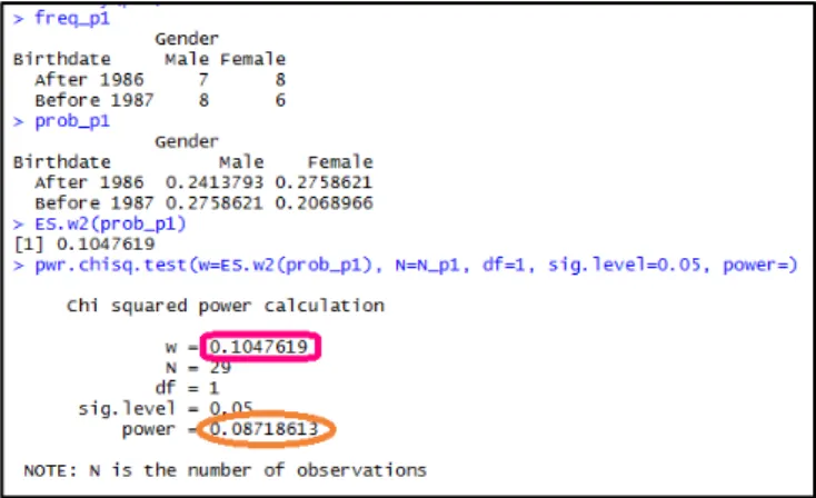
Calculations of w and 1-β for the chi-square test for the preliminary Physiosensor frequency dataset in R software are shown in Figure A2. The structure is similar to that in Figure A1. We used freq_p1 object in this short R script for the contingency table, which is to be seen in Table A3, and prob_p1 object to calculate the probabilities for the overall 29 cases. R calculated the same w and 1-β as generated by GPower software (colored the same in the outputs of the two softwares:
magenta indicates w=0.105, and orange indicates 1-β
=0.087; Figure 4).
FIG. A2 EFFECT SIZE (MAGENTA-FRAMED) AND POWER (ORANGE-FRAMED) CALCULATION FOR PRELIMINARY PHYSIOTHERAPEUTIC DATASET (N=29) IN R SOFTWARE.
The SAS code for power analysis with different sample sizes based on the group proportions of the 2×2 contingency table of the preliminary Physiosensor dataset for the extended dataset (N=34) is to be seen in Figure A3.
FIG. A3 SAS CODE FOR POWER ANALYSIS FOR A 2×2 CONTINGENCY TABLE BASED ON THE PRELIMINARY PHYSIOTHERAPEUTIC DATASET. THE POWER IS CALCULATED ON THE BASIS OF THE PROPORTIONS IN THE PRELIMINARY DATASET, BUT RUN FOR
NUMBER OF CASES (N=34) FROM THE EXTENDED DATASET.
The power calculation in R, using effect size based on the preliminary physiotherapeutic data for the extended (N=34) dataset, is presented in Figure A4. The analysis results in 1-β=0.0937.
FIG. A4 POWER ANALYSIS BASED ON w=0.105 FROM THE PRELIMINARY DATA FOR THE EXTENDED (N=34) DATASET.
1-β=0.0937, CALCULATION WAS PERFORMED IN R.
Study 3: Anthropometric Data
The contingency table of the anthropometric dataset from 2010, comparing waist and hip circumference groups, is shown in Table A5 (total number of cases 362). Each cell contains the number of observed cases, the expected value and the row percentage of each pair of comparisons. This contingency table was created with IBM SPSS Statistics 20.
TABLEA5 CONTINGENCYTABLEFORTHE
ANTHROPOMETRICDATASETCOMPARINGTHEWAISTAND HIPCIRCUMFERENCECATEGORIES(N=362).
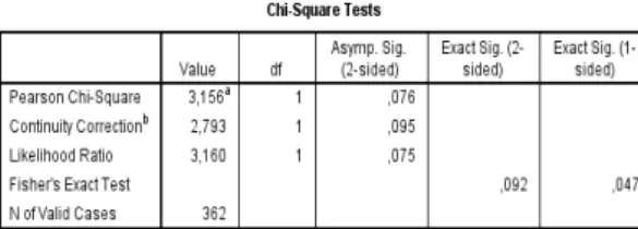
Table A6 results of the chi-square tests on the anthropometric dataset are from 2010. Pearson’s chi- square test shows an asymptotic p-value of 0.076. As none of the cells in the contingency table contains an expected value less than 5, this chi-square test can be interpreted. This table was made with IBM SPSS Statistics 20.
TABLEA6RESULTSOFCHI-SQUARETESTSINSPSSBASEDON THECONTINGENCYTABLESHOWNINTABLEA5.
APPENDIX II
An MS Excel calculator for Effect Size for chi-square power analysis for 2×2, 2×3 and 2×4 contingency tables is available online (http://www3.szote.u- szeged.hu/dmi/Anna_Laszlo/Effect-
size_calculator_for_Chi-square_power.xlsx).
APPENDIX III
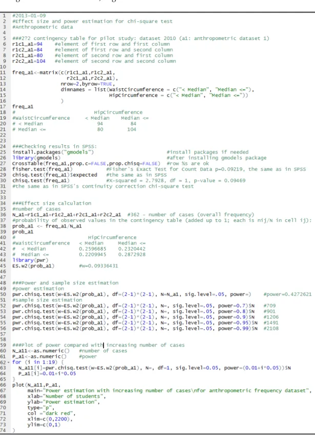
As a third appendix, an R script with explanatory comments for effect size and power estimation of the anthropometric data is available in Figure A5. The code has 5 main parts (indicated by ### at the beginning of the comment):
1. Creating the contingency table (freq_a1 2×2 matrix) by waist and hip circumference groups.
Basically, the user only has to set frequencies for this contingency table, using r1c1_a1, r1c2_a1, r2c1_a1, r2c2_a1 as the number of each cell (counts), where r and c are denoted as row and column, and the numbers indicate, which row and column we are in. For example, r2c1 is the cell at the intersection of the second row and the first column in the contingency table.
The notation “_a1” denotes that these count numbers are from a preliminary study.
2. Running the chi-square test and comparing the results with those from IBM SPSS Statistics (Appendix I; Tables of Study 3) to check the calculations of this software. Contingency table is compared by using the CrossTable() function from the gmodels package. The chi-square test assumption is checked by calculating the expected values from the contingency table.
Fisher’s Exact test and the chi-square test with the Yates continuity correction are compared between the two softwares. They give the same result.
3. For the effect size calculation for the chi-square test, probabilities have to be calculated (prob_a1 2×2 matrix) and the pwr package has to be imported to allow use of the ES.w2() function for effect size estimation.
4. Power is estimated with the pwr.chisq.test() function from the pwr package. To run this estimation, effect size (from the previous calculation by the ES.w2() function), degrees of freedom for the contingency table ((number of rows - 1)*(number of columns - 1)), number of
cases (N_a1 is the sum of the elements in the contingency table) and significance level (α set as 0.05) have to be set. If power is set instead of number of cases, then it can be estimated that how many cases would present a determined value of power (e.g. 0.8, 0.9 and 0.95), supposing the same effect size, significance
level and degrees of freedom.
5. A dot plot was drawn representing the power with increasing number of cases for the same study parameters (w=0.09336431, α=0.05 df=1 as we have a 2×2 contingency table). This is shown in Figure 8.
FIG. A5 R SCRIPT FOR EFFECT SIZE AND POWER CALCULATION FOR THE ANTHROPOMETRIC DATASET