Local stability implies global stability for the 2-dimensional Ricker map
Ferenc A. Bartha†‡, ´Abel Garab‡and Tibor Krisztin∗‡?
†CAPA group, Department of Mathematics, University of Bergen, Bergen, Norway
‡Bolyai Institute, University of Szeged, Szeged, Aradi v. tere 1, 6720, Hungary
?Analyis and Stochastics Research Group of the Hungarian Academy of Sciences,, Bolyai Institute, University of Szeged
Abstract
Consider the difference equation xk+1=xkeα−xn−d whereα is a positive parameter and d is a nonnegative integer. The case d=0 was introduced by W.E. Ricker in 1954. For the delayed versiond≥1 of the equation S. Levin and R. May conjectured in 1976 that local stability of the nontrivial equilibrium implies its global stability. Based on rigorous, computer aided calculations and analytical tools, we prove the conjecture ford=1.
Keywords: global stability; rigorous numerics; Neimark–Sacker bifurcation; graph representa- tions; interval analysis; discrete-time single species model
2010 Mathematics Subject Classification: 39A30, 39A28, 65Q10, 65G40, 92D25
1 Introduction
In 1954, Ricker [21] introduced the difference equation
xk+1=xkeα−xk (1.1)
with a positive parameterα to model the population density of a single species with non-overlapping generations. The functionR1:R3x7→xeα−x ∈Ris called the 1-dimensional Ricker map. R1 has two fixed points: 0 andα. It is not difficult to show thatx=α is stable if and only if 0<α≤2, and, for 0<α≤2,x=αattracts all points from(0,∞); or equivalently, the equilibriumx=αof equation (1.1) is globally stable provided it is locally stable.
In 1976, Levin and May [14] considered the case when there are explicit time lags in the density dependent regulatory mechanisms. This leads to the difference-delay equation of orderd+1:
xk+1=xkeα−xk−d, (1.2)
∗Corresponding author. Email: krisztin@math.u-szeged.hu
arXiv:1209.2406v1 [math.DS] 11 Sep 2012
wheredis a positive integer.
The map
Rd+1:Rd+13(x0, . . . ,xd)T7→(x1, . . . ,xd,xdeα−x0)T∈Rd+1
is called the(d+1)-dimensional Ricker map; hereT denotes the transpose of a vector. Rd+1 has 2 fixed points inRd+1:(0, . . . ,0)T and(α, . . . ,α)T. Levin and May [14] conjectured in 1976 that local stability of the fixed point(α, . . . ,α)T ∈Rd+1implies its global stability in the sense that all points fromRd+1+ := (0,∞)d+1are attracted by(α, . . . ,α)T. As far as we know, the conjecture is still open for all integersd≥1. The aim of the present paper is to prove the conjecture ford=1.
Levin and May’s conjecture and many other numerical and analytical studies suggested the folk theorem that ‘The local stability of the unique positive equilibrium of a single species model implies its global stability.’ This claim was recently disproven by a counterexample of Jim´enez L´opez [11, 12]
on global attractivity for Clark’s equation [4] when the delay is at least 3.
Liz, Tkachenko and Trofimchuk [17] proved that if 0<α< 3
2(d+1) (1.3)
then the fixed point(α, . . . ,α)T ∈Rd+1 of Rd+1 is globally asymptotically stable, where globally means that the region of attraction of(α, . . . ,α)T isRd+1+ . They also suggested that condition (1.3) can be replaced by
0<α< 3
2(d+1)+ 1
2(d+1)2, (1.4)
which was proven by Tkachenko and Trofimchuk in [24]. This result is a strong support of the conjecture of Levin and May, and it is proven for a class of maps, not only for Rd+1. For the 1- dimensional Ricker mapR1, condition (1.4) withd=0 gives the region 0<α<2. Ford=1, i.e., for the 2-dimensional Ricker mapR2, condition (1.4) is equivalent to 0<α<0.875. See also [16]
and [15] in the topic.
LinearisingR2at the fixed point(α,α)Tshows that local exponential stability of(α,α)Tholds for 0<α<1, and(α,α)T is unstable forα>1. Asαpasses the value 1, a Neimark–Sacker bifurcation takes place at the nontrivial fixed point. In this paper we show that global asymptotic stability is true also for the parameter valuesα∈[0.875,1]. We emphasise that our result implies global stability at the critical parameter valueα=1 as well.
In cased=1 the difference equation (1.2) is equivalent to the 2-dimensional system xk+1=yk,
yk+1=ykeα−xk,
(1.5) and this is also equivalent to the 2-dimensional discrete dynamical system generated by the 2-dimensi- onal Ricker mapR2. Asd=1 will be fixed in the remaining part of the paper, we shall use the notation Fαinstead ofR2=R2(α).Fαhas two fixed points(0,0)Tand(α,α)T. From now on, we shall analyse the dynamics generated byFαin the positive quadrantR2+= (0,∞)×(0,∞). Note thatFα(R2+)⊆R2+
andFα(R2+)⊂R2+.
We shall use a combination of analytic and computational arguments. The latter is done using interval arithmetics, that is a standard in the area of validated or rigorous numerics. Instead of calcu- lating with numbers, we use intervals to control the errors introduced by the computer. After finishing a computation, the information we obtain is that the true result is contained in the result interval. We shall draw conclusions from that. An interval[a]is represented as a pair of endpoints[a−,a+]. Having a setSor a numberr, we denote their interval enclosures by [S]and[r], respectively. The reader is referred to Moore [19], Alefeld [2], Tucker [25], [26], Nedialkov, Jackson and Corliss [20] for further details.
The structure of the paper is as follows. In Section 2 we construct a compact regionS, which is a closed square around(α,α)T, having the property thatFα(S)⊆Sand every trajectory enters it eventually. In Section 3 we construct an attracting neighbourhood of the fixed point(α,α)T. We use two different approaches. First, the linear approximation ofFαis applied at the fixed point. Naturally, the size of this neighbourhood tends to 0 as the parameterα tends to the critical value 1. Then we analyse the normal form ofFα used in the study of the Neimark–Sacker bifurcation, and obtain a uniform neighbourhood in the parameter rangeα ∈[0.999,1]belonging to the basin of attraction of the nontrivial fixed point(α,α)T. In addition to the standard techniques applied in the Neimark–
Sacker bifurcation, we need explicit estimations on the sizes of the higher order terms in order to get a sufficiently large attracting neighbourhood of the fixed point (α,α)T. In Section 4 we give an overview on graph representations of discrete dynamical systems and show how it can be used to study qualitative properties of dynamical systems. For possible future applications we formulate two approaches for general continuous maps in Euclidean spaces. In particular, the correctness of an algorithm is verified in order to enclose non-wandering points. In Section 5 we combine the computational techniques of Section 4 and rigorously show that every trajectory ofFα starting from R2+ enters the neighbourhood constructed in Section 3. This proves our main result:
Theorem 1.1. If0<α ≤1, then(α,α)T is locally stable, and Fαn(x,y)→(α,α)T as n→∞for all (x,y)T ∈R2+.
For the sake of completeness, here we give a proof for allα ∈(0,1]. The result is new only for α∈[0.875,1].
There is an appendix containing some large formulae used in Section 3. The program codes and results of our rigorous computer aided computations can be found on link [1].
Consideration of a bifurcation of a given dynamical system is usually used to show that some phenomenon appears in the global dynamics of the system as a parameter passes a critical value.
The invention in our method is that we use the normal form of a bifurcation in combination with the tools of graph representations of dynamical systems and interval arithmetics to prove the absence of a phenomenon for certain parameter values near the critical one. As we want to construct explicitly given and computationally useful regions, the key technical difficulty is the estimation of the sizes of the higher order (error) terms in the normal forms. We hope that our proof shows that these ideas are applicable for a wide range of discrete or continuous dynamical systems, as well.
Running the program of D´enes and Makay [8], which is developed to (nonrigorously) find and
visualise attractors and basins of discrete dynamical systems, suggests that the conjecture of Levin and May stands for the 3-dimensional Ricker model, as well. In order to prove the conjecture in this case and also for larger values ofd, an additional technical difficulty arises. Namely, first a center manifold reduction is necessary, and the construction of an attracting neighbourhood should be done on the center manifold. Among others, an explicit estimation of the size of the center manifold will play a crucial role as well.
Notations and definitions
Throughout the paper some further notations and definitions will be used. N, N0, R, Cstand for the set of positive integers, non-negative integers, real numbers, and complex numbers, respectively.
The open ball in the Euclidean-normk.kand in the maximum norm with radiusδ ≥0 aroundq∈ Rn are denoted by B(q;δ) and K(q;δ), respectively. In Section 3 we shall often use the notation Bδ ={z∈C: |z|<δ}forδ >0, where|z|denotes the absolute value ofz∈C. For a vectorx∈Cn, xT denotes the transpose ofx. For ξ = (ξ1,ξ2)T ∈C2andζ = (ζ1,ζ2)T ∈C2let hξ,ζidenote the scalar product of them defined byhξ,ζi=ξ1ζ1+ξ2ζ2. Let alsoα = (α,α)T.
Let f :Df ⊆Rn→Rnbe a continuous map. Fork∈N0, fk denotes thek-fold composition of f, i.e., fk+1(x) = f(fk(x)), and f0(x) =x. A fixed point p∈Df of f is called locally stable if for every ε>0 there existsδ >0 such thatkx−pk<δ implies kfn(x)−pk<ε for alln∈N. We say that the fixed point pattracts the regionU ⊆Df if for all pointsu∈U,kfn(u)−pk→0 asn→∞. The fixed pointpis globally attracting if it attracts all ofDf and is globally stable if it is locally stable and globally attracting.
2 The dynamics in the first quadrant
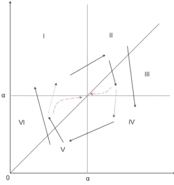
In this section we construct compact squaresS(α)i ⊂R2+,i∈N0aroundα so thatFα(S(α)i )⊆Si(α)and S(α)i attracts all points ofR2+for alli∈N0andα ∈(0,1]. Hence an elementary proof of Theorem 1.1 is obtained for 0<α≤0.5. RecallFα(R2+)⊆R2+. We can illustrate the image(xk+1,yk+1)of(xk,yk) as first going horizontally from(xk,yk)to the diagonal, proceeding upwards if 0<xk<α, otherwise downwards vertically until we reach the valueyk+1=ykeα−xk. This is shown on Figure 1.
Figure 1: Dynamics forx>0,y>0
Let(x0,y0)∈R2+ and 0<α ≤1 be given. Define the sequence(xk,yk)∞k=0∈R2+by (xk+1,yk+1) =Fα(xk,yk),k∈ {0,1, . . .}.
Consider the following cases:
I. 0<x0≤α≤y0
Clearly we haveα ≤x1≤y1and max{x0,y0,x1,y1} ≤y1. II. α≤x0≤y0
In this caseα≤x1andy1≤x1with max{x0,y0,x1,y1} ≤y0. We distinguish two cases depending ony1≤α or not.
III. α≤y0≤x0
We obtainα≤y0=x1 andy1≤y0=x1. During the consequent iterationsyi+1≤yi=xi+1 is satisfied as long asα ≤xistays true. Ifα≤xifor alli, thenyi>0 for alli, and both(yi)∞i=0and (xi)∞i=0 are monotonically decreasing, and converge. The only possibility is(xk,yk)→(α,α), since the other fixed point is at(0,0). Otherwise there is a minimalN>0 such that 0<yN ≤ xN<αis satisfied. We note that 0<yN−1<α≤xN−1is true. We have maxi∈{0,...,N}{xi,yi}<x0. IV. 0<y0<α≤x0
Obviously 0<y1≤x1<α, and max{x0,y0,x1,y1} ≤x0. V. 0<y0≤x0≤α
Here we have 0<x1≤α, 0<x1≤y1 and max{x0,y0,x1,y1} ≤y1. We distinguish two cases depending onα ≤y1or not.
VI. 0<x0≤y0≤α
Thenx1≤α andx1 ≤y1. Now xi+1=yi ≤yi+1 is satisfied as long as xi≤α stays true. If xi≤α for alli, thenyi>0 for alli, and both(yi)∞i=0and(xi)∞i=0are monotonically increasing, and converge. The only possibility is(xk,yk)→(α,α), since the other fixed point is at(0,0).
Otherwise there is a minimalN>0 such thatα<xN≤yNis satisfied. We note that 0<xN−1≤ α<yN−1. We have maxi∈{0,...,N}{xi,yi}<yN.
We conclude that for any(x0,y0)∈R2+ the sequence((xk,yk))∞k=0 converges to(α,α)or enters the triangle H(h(α)0 ) ={(x,y):h(α)0 <y≤x≤α}, withh(α)0 =0, that is the region denoted by V in Figure 2. We mark the possible transitions with arrows, if it is solid, it refers to transition in one step, otherwise it is possible to have multiple iterations before entering the next region.
Figure 2: Dynamics forx>0,y>0
Assume now that(x0,y0)∈H(h(α)0 ). Either the sequence converges to (α,α)or there exists an N>1 such that(xN−1,yN−1)∈V∪V I,(xN,yN)∈Iand(xN+1,yN+1)∈II. So the following stands:
yN+1=yNeα−xN=yN−1e2α−xN−xN−1 ≤αe2α−2h
(α)
0 .
This implies that(xN+1,yN+1)∈G(g(α)0 ), whereG(g(α)0 ) ={(x,y):α ≤x≤y≤g(α)0 }, withg(α)0 = αe2α−2h(α)0 . Now there exists M ≥N+2 such that (xM−1,yM−1)∈ II∪III, (xM,yM) ∈IV and (xM+1,yM+1)∈V. We get the following inequality:
yM+1=yM−1e2α−xM−xM−1 ≥αe2α−2g(α)0 .
Therefore(xM+1,yM+1)∈H(h(α)1 ), with h(α)1 =αe2α−2g(α)0 . Similarly, the sequence will enter the setG(g(α)1 ), withg(α)1 =αe2α−2h(α)1 . Repeating this argument we get two sequences (h(α)i )∞i=0 and
(g(α)i )∞i=0defined recursively byh(α)0 =0,h(α)i =αe2α−2g(α)i−1 fori≥1, andgi=αe2α−2h(α)i fori≥0.
It is easy to see that(h(α)i ) increases and(g(α)i )decreases. We have the limitsh(α)i %h(α)∞ ≤α and g(α)i &g(α)∞ ≥α. Define
S(α)i ={(x,y):h(α)i ≤x≤g(α)i ,h(α)i ≤y≤g(α)i }. (2.1) We sum our observations in the following Lemma:
Lemma 2.1. For everyα ∈(0,1]and for every i∈N0
1. Fα(S(α)i )⊆S(α)i ,
2. S(α)i attracts all points ofR2+.
IfS(α)∞ ={(α,α)}, then we have already established that the fixed point is globally attracting.
This is not the case however forα>0.5. For a givenα, we can view the sequences(h(α)i )and(g(α)i ) as even and odd iterates of the function
τα(t) =αe2α−2t, (2.2)
starting fromt=0. That is,h(α)0 =τα0(0), g(α)0 =τα1(0),h(α)1 =τα2(0),g(α)1 =τα3(0), . . . .The non- rigorous bifurcation diagram on Figure 3 shows that the unique fixed pointα ofτα is stable for 0<
α<0.5, it is unstable forα>0.5, and there is an attracting 2-cycle forα>0.5. ThusS(α)∞ ={(α,α)}
can be expected only forα ∈(0,0.5). Forα>0.5 the two points of the 2-cycle giveh(α)∞ andg(α)∞ .
Figure 3: Bifurcation diagram ofτα
Proposition 2.2. If0<α≤0.5, then for every(x,y)∈R2+we have Fαn(x,y)→(α,α)as n→∞.
Proof. Observe thatτα0(t) =−2τα(t),τα(t)>0, and ift>α andα ∈(0,0.5], then 2τα(t) =2α≤1 is satisfied. Since
d2
dt2(τα(τα(t))−t) =8τα(τα(t))τα(t) (2τα(t)−1), (2.3)
thereforeτα(τα(t))−tis a concave function fort>α. The first derivative atα ∈(0,0.5]is d
dt(τα(τα(t))−t) t=α
=4τα(τα(α))τα(α)−1=4α2−1≤0. (2.4) These imply thatdtd (τα(τα(t))−t)<0 for allt>α. Thus the only zero ofτα(τα(t))−tint∈[α,∞) isα. This gives us thatg(α)∞ =α which implies thath(α)∞ =α and consequentlyS(α)∞ ={(α,α)}in this parameter region.
We assumeα ∈[0.5,1]in the remaining part of the paper.
3 Attracting neighbourhood
Let us consider map Fα. In this section we are going to give ε(α) > 0, such that infα∈[0.5,1]ε(α)>0 and K(α;ε(α)) belongs to the basin of attraction of α for α ∈[0.5,1], that is,Fαn(x0,y0)→α asn→∞for all(x0,y0)T ∈K(α;ε(α)).
Introducing the new variablesu=x−α,v=y−α, mapFα can be written in the form u
v
!
7→A(α) u v
!
+fα(u,v), (3.1)
where the linear part is
A(α) = 0 1
−α 1
!
and the remainder is
fα(u,v) = 0
v(e−u−1) +α(e−u−1+u)
! .
The eigenvalues ofA(α)areµ1,2(α) = 1±i
√4α−1
2 ∈C, and the corresponding complex eigenvectors areq1,2(α) =
1∓√ 1−4α 2α ,1T
=
1∓i√ 4α−1 2α ,1
T
∈C2,respectively for α > 14. Letq(α) =q1(α) andµ(α) =µ1(α). Letp(α)∈C2denote the eigenvector ofA(α)T corresponding toµ(α)such that hp(α),q(α)i=1,. This leads to
p(α) =
− iα
√4α−1,
√4α−1+i 2√
4α−1 T
.
We introduce a complex variable
z=z(u,v,α) =hp(α),(u,v)Ti=1 2
v−i(v−2uα)
√−1+4α
. (3.2)
We also have an explicit formula for(u,v)T in terms ofz, which reads as (u,v)T=zq(α) +zq(α) =
Rez+√
4α−1Imz
α ,2Rez
T
. (3.3)
Our original system (3.1) is now transformed into the complex system z7→G(z,z,α) =D
p(α),A(α)(zq(α) +zq(α)) +fα(zq(α) +zq(α))E
=µ(α)z+g(z,z,α),
(3.4)
wheregis a complex valued smooth function ofz,zandα, defined by (A.1). It can also be seen that for fixedα,gis an analytic function ofzandzand the Taylor expansion ofgwith respect tozandz has only quadratic and higher order terms. That is,
g(z,z,α) =
∑
2≤k+l
1
k!l!gkl(α)zkzl, withk,l=0,1, . . . , wheregkl(α) = ∂z∂kk+l∂zlg(z,z,α)
z=0fork+l≥2, k,l={0,1, . . .}.
Proposition 3.1. Letα ∈[0.5,1)be fixed and
ε(α) =min (
1 20
r4α−1
2+α , 9(4α−1)(1−√ α) 20(1+2√
α)√ 2+α
) .
Then
(x,y)T∈R2:|x−α|<ε(α),|y−α|<ε(α) belongs to the basin of attraction of the fixed pointα of Fα.
Proof. Let us study the map in the form (3.4). First note that (3.3) easily implies inequalities
|u|≤ 2
√ α
|z|and|v|≤2|z|. (3.5)
Assuming |u|<1/10 and |v|<1/10 and applying the inequalities |e−u−1| ≤e1/10|u|≤ 109|u| and
|e−u−1+u| ≤e1/10u22 ≤59u2we obtain the following estimations:
|g(z,z,α)|= D
p(α),fα
zq(α) +zq(α) E
=
√4α−1+i 2√
4α−1
v(e−u−1) +α(e−u−1+u)
≤ r α
4α−1 |v||e−u−1|+α|e−u−1+u|
≤ r α
4α−1 |uv|e1/10+αe1/10 2 u2
!
≤5 9
r α
4α−1 u2+2|uv|)
≤5
9· 4(1+2√ α) pα(4α−1)|z|2. Now, since|µ(α)|=√
α, hence
|G(z,z,α)|≤ √ α+5
9· 4(1+2√ α) pα(4α−1)|z|
!
|z|<|z|
provided that|z|6=0 is so small that|u|<101 and|v|< 101 and√
α+59· 4(1+2
√α)
√α(4α−1)|z|<1. Inequalities (3.5) imply that|z|<
√ α
20 guarantees|u|<101 and|v|<101. Therefore 0<|z|<εG(α) =min
(√ α
20 ,9(1−√ α)p
α(α−1) 20(1+2√
α) )
(3.6) implies|G(z,z,α)|<|z|, which means that|Gn(z0,z0,α)|→0 asn→∞if|z0|<εG(α)is satisfied. We show this by way of contradiction. Assume that|z0|<εG(α),zn=Gn(z0,z0,α)and|z0|>|z1|>· · ·>
|zn|> . . .≥0 with|zn|→c>0 asn→∞. SinceGis continuous we have that max|z|=c|G(z,z,α)|<c and consequently|zk|<calso holds ifkis large enough which is a contradiction.
From equation (3.2) one obtains that if|u|<δ,|v|<δ, then
|z|<δ r
α(2+α)
4α−1 . (3.7)
From (3.7) we infer that if|u|<ε(α) and|v|<ε(α) then |z(u,v,α)|<εG(α) which completes our proof.
Note thatε(α)goes to 0 asαgoes to 1. This means that whenαis close to 1, then the constructed region K(α;ε(α))becomes very small. Thus it is impossible to show by interval arithmetic tools that every trajectory enters into it eventually. Neverthelessε(α)might be used in the caseα∈[0.5,0.999].
However, our following method is not only capable to give an attracting neighbourhood for allα ∈ [0.999,1], whose size is independent of the concrete value of the parameter, but it also serves a better estimation of the attracting region even if we assume onlyα ∈[0.875,1]. The main results of the section are the following two propositions. Here, we only present the proof of Proposition 3.3. The whole argument can be repeated to get a universal attracting neighbourhood when only[0.875,1]is assumed. The differences only appear in concrete values in the given estimations.
Proposition 3.2. For all fixedα∈[0.875,1],
(x,y)T∈R2:|x−α|<1/37,|y−α|<1/37 belongs to the basin of attraction of the fixed pointα of Fα.
Proposition 3.3. For all fixedα∈[0.999,1],
(x,y)T∈R2:|x−α|<1/22,|y−α|<1/22 belongs to the basin of attraction of the fixed pointα of Fα.
Proof. We follow the steps of finding the normal form of the Neimark–Sacker bifurcation, according to Kuznetsov [13]. In our calculations and estimations we use symbolic calculations and built in symbolic interval arithmetic tools of Wolfram Mathematica v. 7 or 8.
According to Kuznetsov [13], we are aiming to transform system (3.4) to a system which takes the following form.
w7→µ(α)w+c1(α)w2w+R2(w,w,α), (3.8) wherec1andR2are smooth, real functions such that for fixedα,R2(w,w,α) =O(|w|4). We are going to show that there existsε0>0 such that for all|w|<ε0andα∈[0.999,1],
µ(α)w+c1(α)w2w+R2(w,w,α) <|w|
holds, which implies that Bε0 belongs to the basin of attraction of the fixed point 0 of the discrete dynamical system generated by (3.8). From this, we shall be able to show that the fixed pointα ofFα attracts all points of K(α;221).
To be more precise, for a fixedα, we are looking for a functionhα :C→C, which is invertible in a neighbourhood of 0∈Cand which is such that in the new coordinatew=h−1α (z), our map (3.4) takes the form
w7→h−1α (G(hα(w),hα(w),α)) =µ(α)w+c1(α)w2w+R2(w,w,α), (3.9)
whereR2(w,w,α) =O(|w|4)for fixedα. According to [13], such a function can be found in the form hα(w) =w+h20(α)
2 w2+h11(α)ww+h02(α)
2 w2+h30(α)
6 w3+h12(α)
2 ww2+h03(α)
6 w3. (3.10) Clearly,hαhas an inverse in a small neighbourhood of 0∈C. A formula forh−1α can be given in the form
h−1α (z) =hinv,α(z) +R3(z,α), where
hinv,α(z) =z+
∑
2≤k+l≤4
akl(α)zkzl
andR3(z,α) =O(|z|5). The coefficients can be obtained by substitutingw=h−1(z)intoz=hα(w) and equating the coefficients of the same type of terms up to the fourth order. The result forhinv,α in terms ofh20(α), . . . ,h03(α)is given in (A.14). The coefficientsh20(α), . . . ,h03(α)are determined such that
h−1α (G(hα(w),hα(w),α))
has the formµ(α) +c1(α)w2wplus at least fourth order terms inw, that is, the transformation kills all second and third order terms with one exception. This requires the condition
µ(1)
|µ(1)|
k
6=1 for allk∈ {1,2,3,4}.
Asµ(1) =12+i
√3
2 , this is clearly satisfied. Formulae (A.15)-(A.20) contain the obtained results.
In which region is the transformation valid? We are going to show thathαis injective on B1/3⊂C and thath−1α is defined on B1/5. Let us suppose thatz∈Cis fixed andh20(α), . . . ,h03(α)are given for a fixedα∈[0.999,1]. Let
Hα,z:C3w7→w+z−hα(w)∈C.
By this notation,Hα,z(w) =wholds if and only ifhα(w) =z. Now, we have the following
|Hα,z(w1)−Hα,z(w2)|=|w1−hα(w1)−w2+hα(w2)|
≤|w1−w2|·
|h20(α)|
2 +|h11(α)|+|h02(α)|
2
(|w1|+|w2|) + |h30(α)|
6 +|h12(α)|
2 +|h03(α)|
6
|w1|2+|w1||w2|+|w2|2
. If|h20(α)|/2+|h11(α)|+|h02(α)|/2<δ1, |h30(α)|/6+|h12(α)|/2+|h03(α)|/6<δ2,|w|≤δ3and
|z|≤δ4hold, then we have
|Hα,z(w1)−Hα,z(w2)| ≤ |w1−w2|(2δ1δ3+3δ1δ32) and
|Hα,z(w)| ≤δ4+δ1δ32+δ2δ33.
By interval arithmetics we obtain that the first two inequalities are fulfilled ifδ1=0.76 andδ2=0.52.
Now, if we chooseδ3= 13 andδ4= 15 we obtain that Hα,z: B1/3→B1/3 is a contraction. Hence
for all fixedz∈B1/5 there exists exactly onew=w(z)∈B1/3 such thatHα,z(w(z)) =w(z), that is hα(w(z)) =z. This means thath−1α can be defined on B1/5.
The obtained estimations onhα are going to be used in the sequel. These were
|h20(α)|/2+|h11(α)|+|h02(α)|/2<0.76,
|h30(α)|/6+|h12(α)|/2+|h03(α)|/6<0.52 and in particular
|w|−0.76|w|2−0.52|w|3<|hα(w)|<|w|+0.76|w|2+0.52|w|3 (3.11) for allα ∈[0.999,1].
Let H ={(α,w)∈R×C: α ∈[0.999,1], w6=0 and|w|<1/20}. In the sequel, we shall always assume that (α,w) ∈H. From this assumption and inequality (3.11) we readily get that
|w|<1.05|hα(w)|from which we get in particular that|z|=|hα(w)|<1/19.
Our goal now is to give ε0∈(0,1/20],independent of α such that for everyα ∈[0.999,1], if 0<|w|<ε0, then
h−1α
G
hα(w),hα(w),α
<|w|holds which guarantees that Bε0belongs to the basin of attraction of the fixed point 0 of the discrete dynamical system generated by (3.9). For, we turn our attention to the estimation of functionR2in (3.9).
First, we go back to (3.4). Let us consider g(z,z,α) =
∑
k+l=2,3
gkl(α)
k!l! zkzl+R1(z,z,α).
The explicit formulae for g20(α), . . . ,g03(α) can be found in equations (A.2)–(A.8). By interval arithmetics, one may obtain that for allα∈[0.999,1],
|g20(α)|
2 +|g11(α)|+|g02(α)|
2 =1−α+p
α(2+α)
pα(−1+4α) <1.01, (3.12)
|g30(α)|
6 +|g21(α)|
2 +|g12(α)|
2 +|g03(α)|
6 =
s
(6+α) 9α(4α−1)+
s
2+ (α−2)α
α2(4α−1) <1.09. (3.13) We also have thatR1(z,z,α) =∑k+l=4
gkl(α)
k!l! zkzl+R˜1(z,z,α), where ˜R1(z,z,α) =O(|z|5)for fixed α. For explicit formulae of the fourth order coefficients see equations (A.9)-(A.13) in the appendix.
It is clear from equations (3.1), (3.3) and (3.4) that R˜1(z,z,α) =
√
4α−1−i 2√
4α−1 v
∞
∑
k=4
(−u)k k! +α
∞
∑
k=5
(−u)k k!
! ,
where u and v are defined by equation (3.3). Using 0<|z|<1/19 and (3.5) we have that |u|<
1/8, |v|<1/8 and obtain
R˜1(z,z,α) ≤
r α
4α−1 |v|e1/8
4! |u|4+αe1/8 5! |u|5
!
<
r α 4α−1
8 7
2|z| 16
24α2+ 32 α3/2120|z|
|z|4
≤ r α
4α−1 8 7
4
57α2+ 4 285α2
|z|4= 64 665
s 1
(4α−1)α3|z|4.
Now for all(α,w)∈H withz=hα(w)we get that
|R1(z,z,α)| ≤
∑
k+l=4
gkl(α) k!l! zkzl
+
R˜1(z,z,α)
=6−3α+p
α(12+α) +4√ 3+α2 12p
α3(−1+4α) +
R˜1(z,z,α)
<4758−1995α+665p
α(12+α) +2660√ 3+α2 7980p
α3(−1+4α) . By interval arithmetics we obtain for allα∈[0.999,1]that
|R1(z,z,α)|<0.76|z|4. (3.14) We also need a similar estimation on
h−1α (z)
. Let us recall thatz=hα(w)and w=h−1α (z) =hinv,α(z) +R3(z,α).
Ashinv,α(z)is a polynomial ofz andzof degree four (see formulae (A.14)–(A.20)), we denote the coefficient corresponding tozkzl byhklinv(α). Calculating these coefficients and using interval arith- metics, we obtain that for allα∈[0.999,1],
∑
k+l=2
hklinv
<0.76,
∑
k+l=3
hklinv
<1.06 and
∑
k+l=4
hklinv
<1.39. (3.15) See formulae (A.21) – (A.27). Let us recall that for all(α,w)∈H,|w|<1.05|hα(w)|holds. Now, for the fifth and higher order terms inR3, first we give an estimation of type|R3(hα(w),α)|<K3|w|4and then we get that|R3(z,α)|<K31.054|z|4, withz=hα(w).
From the definition ofhinv,α, it follows thatR3(hα(w),α) =w−hinv,α(hα(w))is a polynomial of wandwand it has only fifth and higher order terms. Letrkl3(α)denote the coefficient ofR3(hα(w),α) corresponding towkwl. We use a bit rougher estimation for
∑5≤k+lrk+l3 (α)wkwl
. Namely, first we give the estimations
|h20(α)|<1.01; |h11(α)|<0.001; |h02(α)|<0.51
|h30(α)|<0.89; |h12(α)|<0.45; |h03(α)|<0.89
(3.16) for allα ∈[0.999,1]. Now, inR3(hα(w),α) we replacew andw by |w|, hnm(α) by the estimates given in (3.16) (for 2≤n+m≤3,(n,m)6= (2,1)), and then we turn every−sign into+to get a real polynomial ˆR3(|w|), with nonnegative coefficients ˆrk3(independent ofα) corresponding to|w|k. If we use 0<|w|<1/20, then we get that
5≤k+l≤12
∑
|rkl3(α)||w|k+l<
∑
5≤k≤12
ˆ
r3k|w|k<
∑
5≤k≤12
ˆ rk3|w|4
1 20
k−4
<1.02|w|4. (3.17) This implies that
|R3(z,α)|<1.054·1.02|z|4<1.24|z|4 (3.18) for all(α,w)∈H, wherez=hα(w). It is now clear that
hinv(z)<|z|+0.76|z|2+1.06|z|3+2.63|z|4 (3.19) holds for all(α,w)∈Hwithz=hα(w).
Now, we are able to give an estimation onR2in (3.9). First, according to our previous estimations, let us define the following real polynomials.
hmax(s) =s+0.76s2+0.52s3, Gmax(s) =s+1.01s2+1.09s3+0.76s4,
hmaxinv (s) =s+0.76s2+1.06s3+2.63s4 and
Q(s) =
48
∑
k=1
qk(s) =hmaxinv ◦Gmax◦hmax(s).
By now, it is obvious that for(α,w)∈H,|R2(w,w,α)|<∑48k=4qk(|w|)|w|4 201k−4
holds, which leads to|R2(w,w,α)|<23.9|w|4. For our purposes this approach is too rough – the obtained neighbourhood would be too small(≈K(α; 1/80))and we could not prove that every trajectory enters it eventually.
Hence we have to be as sharp as we can in our estimations to obtain as large neighbourhood as possible. So, instead of only estimating these functions separately, let us consider the composite functionh−1α ◦Gα◦hα, whereGα(z)denotesG(z,z,α). Now, we are only interested in the fourth and higher order terms. Sincehαis a known function and we also know functionsGαandh−1α up to fourth order terms, hence we are able to compute the fourth order coefficients ofh−1α ◦Gα◦hα, denoted by rkl2(α), wherek+l=4. By interval arithmetics we show that
∑
k+l=4
|rkl2(α)|<1.02. (3.20)
See equations (A.28) – (A.32) for the formulae. Using this we infer that
|R2(w,w,α)|<1.02|w|4+
48
∑
k=5
qk|w|4 1
20 k−4
<4.6|w|4. (3.21) for all(α,w)∈H.
Now, we turn our attention toc1(α)in (3.9). The formula forc1(α)can be found in (A.33).
According to [13] and using inequality (3.21) we get the following µ(α)w+c1(α)w2w+R2(w,w,α)
≤ |w|
µ(α) +c1(α)|w|2
+|R2(w,w,α)|
=|w|
|µ(α)|+d(α)|w|2
+|R2(w,w,α)|<|w|
√
α+d(α)|w|2
+4.6|w|4,
(3.22)
for all(α,w)∈H, whered(α) =|µ(α)|µ(α)c1(α). Let R4(w,α) =
√
α+d(α)|w|2 −(√
α+a(α)|w|2), wherea(α)denotes the real part ofd(α).
In the following we are going to prove that|R4(w,α)|<0.1|w|3holds for all(α,w)∈H. First of all, the formula for functionais the following
a(α) = 4+α −10+α+α2
4α3/2(−1+α(4+α)). (3.23)
It can be readily shown that
−1<a(α)≤ −1
4 (3.24)
holds for allα∈[0.999,1]. Using the definition ofd anda, the estimation above and the assumption (α,w)∈Hwe get the following.
√
α+d(α)|w|2 −(√
α+a(α)|w|2) =
q
α+2√
αa(α)|w|2+|d(α)|2|w|4−(√
α+a(α)|w|2)
=
(|d(α)|2−(a(α))2)|w|4 p
α+2√
αa(α)|w|2+|d(α)|2|w|4+√
α+a(α)|w|2
≤ (|d(α)|2−(a(α))2)|w|4 p400α|w|2+2√
αa(α)|w|2+20√
α|w|+a(α)|w|≤ (|d(α)|2−(a(α))2)
√
400α−2+20α−1|w|3
≤(|d(α)|2−(a(α))2) 19√
α+18α · |w|3≤(|d(α)|2−(a(α))2)
37α · |w|3= α4+3α3−12α2+20α−42
16·37α6(4α−1)(α2+4α−1)2· |w|3. From this last formula it can be proven that|R4(w,α)|<0.1|w|3. From inequalities (3.22), (3.24) and from the above estimate we obtain that for all(α,w)∈Hthe inequalities
µ(α)w+c1(α)w2w+R2(w,w,α)
<|w| √
α+a(α)|w|2+R4(w,α)
+4.6|w|4
<√
α|w|−1
4|w|3+4.7|w|4<|w|
1−1
4|w|2(1−4·4.7|w|)
<|w| (3.25)
hold provided that |w|< 201 =min1
20,4·4.71 . This means that for all α ∈[0.999,1]the set B1/20 belongs to the basin of attraction of the discrete dynamical system generated by (3.9).
Now, we only have to show that for any(x,y)T ∈K(α; 1/22), after our transformations, |w|<
ε0=201 holds. First, we needεGsuch that for|z|<εG,|w|=|h−1α (z)|<201 holds for allα∈[0.999,1].
From (3.11) we obtain thatεG=211 is an appropriate choice. Now, if|u|<ε, |v|<ε, then from (3.7) we get that
|z(u,v,α)|≤ε r
α(2+α) 4α−1 . Thus for
ε< min
α∈[0.999,1]
s
4α−1 α(2+α)· 1
21 (3.26)
we get that if|u|<ε and|v|<ε then|z(u,v,ε)|< 211. It is easily shown thatε =221 fulfils inequality (3.26) which proves our proposition.
Proposition 3.4. Fixed pointαof map Fαis locally asymptotically stable if and only ifα∈(0,1].
Proof. By linearisation one readily gets that α is locally asymptotically stable if α ∈(0,1), and unstable ifα ∈(1,∞). Transforming mapFαto the form (3.9) and using inequality (3.25) yields that 1 is a locally asymptotically stable fixed point ofF1.
4 Graph representations
Covers and graph representations
Different directed graphs can be associated with a given map. The graphs reflect the behaviour of the map up to a given resolution. The vertices of these graphs are sets and the edges correspond to transitions between them. We can derive properties of our dynamical system through the study of the graphs. These techniques appeared in many articles, in both rigorous and non-rigorous computations for maps by Hohmann, Dellnitz, Junge, Rumpf [6], [7], Galias [9], Luzzatto and Pilarczyk [18], and computations for the time evolution of a continuous system with a given timestep by Wilczak [27].
We introduce the general setting and two applications in particular. One to enclose the non-wandering points and the other one to estimate the basin of attraction.
Both methods (Algorithms 1 and 2) combined with local estimations of the type of Section 3 at the critical points, can be theoretically applied to prove different dynamical properties. On the one hand these algorithms are included for possible future references, on the other hand certain elements of these algorithms proved to be useful for the mapFα in Section 5. In particular, the correctness of Algorithm 1 is crucial in Section 5.
Definition 4.1. S is called acoverofD⊆Rnif it is a collection of subsets ofRnsuch that∪s∈Ss⊇ D. We denote their union∪s∈Ssby|S|in the following. We define thediameterorouter resolution of the coverS by
R+(S) =diam(S) =sup
s∈Sdiam(s).
with
diam(s) =sup
x,y∈s
kx−yk.
A coverS2is said to befinerthan the coverS1if
(∀s1∈S1) (∃{s2,i,i∈I} ⊆S2) such that [
i∈I
s2,i=s1.
We denote this relation byS24S1. Theinner resolutionof a coverS is the following:
R−(S) =sup{r≥0 :∀x∈D,∃s∈S : B(x;r)⊆s}.
A cover S is essential ifS \s is not a cover anymore for anys∈S. The cover P is called a partitionif it consists of closed sets such that|P|=Dand∀p1,p2∈P:p1∩p2⊆bd(p1)∪bd(p2), where bd(p) is the boundary of the set p. Consequently, for any partition P the inner resolution R−(P)is zero.
In the following we will always work with essential and finite partitions, as a consequence the supremum in the definition of the diameterR+of the partition becomes a maximum.
Definition 4.2. Adirected graphG =G(V,E)is a pair of sets representing the verticesV and the edgesE, that is:E ⊆V ×V, and(u,v)∈E means thatG has a directed edge going fromutov. We
say thatv1→v2→. . .→vk is adirected pathif(vi,vi+1)∈E for alli=1, . . . ,k−1. Ifvk=v1, then it is adirected cycle.
A directed graphG is calledstrongly connectedif for anyu,v∈V,v6=uthere is a directed path fromutovand fromvtouas well. Thestrongly connected components(SCC) of a directed graph G are its maximal strongly connected subgraphs. It is easy to see thatuandvare in the same SCC if and only if there is a directed cycle going through bothuandv. Every directed graphG, can be decomposed into the union of strongly connected components and directed paths between them. If we contract each SCC to a new vertex, we obtain a directed acyclic graph, that is called thecondensation ofG.
We say that the directed paths p1,p2 are from the samefamily of directed paths, if they visit the same vertices inV (multiple visits are possible). If the set of the visited vertices isV ⊆V, then we denote the family byϒpath(V), and we say thatV is thevertex set of the family. In a similar manner we can define thefamily of directed cycles, and denote it byϒcycle(V), and say thatV is the vertex set of the family.
Definition 4.3. Let f :Df ⊆Rn→Rn,D ⊆Df, andS be a cover ofD. We say that the directed graph G(V,E) is a graph representation of f on D with respect to S, if there is a ι :V →S bijection such that the following implication is true for allu,v∈V:
f(ι(u)∩D)∩ι(v)∩D6=/0⇒(u,v)∈E, and we denote it byG ∝(f,D,S).
Having a graph representation G of f on D with respect to S, we take the liberty to handle the elements of the cover as vertices and vica versa, omitting the usage of ι. It is important to emphasise that in general(u,v)∈E does not imply that f(u∩D)∩v∩D 6=/0. If we have(u,v)∈ E ⇔ f(u∩D)∩v∩D6=/0, then we callG anexactgraph representation.
Enclosure of the non-wandering points Consider the continuous map
f :Df ⊆Rn→Rn (4.1)
Let f−1(x) ={y∈Df : f(y) =x}, forx∈Rn.
Definition 4.4. The pointq∈Df is called afixed pointif f(q) =q. q∈Df is aperiodic point with minimal period mif fm(q) =qand for all 0<k<m:fk(q)6=q;q∈Df iseventually periodicif it is not periodic, but there is ak0such that fk0(q)is periodic. The pointq∈Df is anon-wandering point of f if for every neighbourhoodU ofqand for anyM≥0, there exists an integerm≥Msuch that
fm(U∩Df)∩U∩Df 6=/0.
LetK⊆Df be a compact set. We denote the set of periodic points of f inKby Per(f;K)and the set of non-wandering points of f inKby NonW(f;K).
Instead of directly studying the map (4.1), we will analyse different graph representations of f. LetK⊆Df be a compact set satisfying f(K)⊆K,Pa partition ofK, andG ∝(f,K,P). We shall use the algorithm from [9] to enclose the non-wandering points inK.
Algorithm 1Enclosure of non-wandering points
1: functionENCLOSURENONW(f,K,δ0) . f is the function,Kis the starting region.
2: k←0
3: V0←Partition(K,δ0) .V0is a partition ofK, diam(V0)≤δ0.
4: loop
5: Ek←Transitions(Vk,f) .The possible transitions (extra edges may occur).
6: Gk←GRAPH(Vk,Ek) .Gk∝(f,|Vk|,Vk)
7: for allv∈Vkdo
8: ifvisnotin a directed cyclethen
9: removevfromGk
10: end if
11: end for
12: ifGkis emptythen
13: return /0 .There is no non-wandering point inK⇒NonW(f;K) =/0.
14: else
15: δk+1←δk/2
16: Vk+1←Partition(|Vk|,δk+1) .Vk+1is a partition of|Vk|, diam(Vk+1)≤δk+1
17: k←k+1
18: end if
19: end loop
20: end function
However, this algorithm for enclosing non-wandering points appeared without a full proof. We will give it here, not just for the sake of completeness, but because some steps are non-trivial. We need to take special care when a non-wandering point is on the boundary of a partition element.
For anyx∈K, define
P˜x:={u∈P:x∈u}.
Since we are working with finite covers, bothPand ˜Px are finite.
Lemma 4.5. For every q∈K, there is anηq>0such that for any u∈P, if u∩B(q;ηq)6=/0, then q∈u.
Proof. Since we are working with finite partitions, this is very easy to see. If P˜q=P then any positive number satisfies the condition. Otherwise define
η:= min
u∈P\P˜q
d(q,u).
This is positive, sinceP\P˜qis a finite set and foru∈P\P˜q,uis compact andq∈/u. Now we can take any number forηqfrom(0,η).
Lemma 4.6. For every q∈NonW(f;K), there are u,v∈Psuch that 1. q∈u∩v
2. for everyε >0, there are x=x(ε),N=N(x(ε),ε)∈Nsuch thatlimε→0N(x(ε),ε) =∞, x∈ B(q;ε),fN(x)∈B(q;ε), x∈u and fN(x)∈v.
Proof. Consider a decreasing sequence of positive numbers{εk}∞k=0with limk→∞εk=0 andε0<ηq. Sinceqis non-wandering,
∃Nk≥k: fNk(B(q;εk)∩Df)∩B(q;εk)∩Df 6=/0.
Therefore
∃xk∈B(q;εk): fNk(xk)∈B(q;εk).
Since ˜Pqis finite, we can picku∈P˜qsuch that it contains infinitely manyxk-s. We may assume, by switching to an appropriate subsequence and reindexing, that∀k:xk∈u. It is now possible to choose – because of finiteness again – an element of the partitionv∈P˜qsuch that it contains infinitely many of fNk(xk). Switching again to the subsequence, the required conditions are now satisfied.
Remark4.7. If there existsu∈Psuch thatq∈int(u)then it follows from the definition, thatuand v=uis a good choice. By int(u)we mean the interior of the setu.
Lemma 4.8. For every q∈NonW(f;K)\Per(f;K) there is an element u∈P˜q and a family of directed cyclesϒcycle(V)inG such that u∈V , and the family encloses infinitely many trajectories in K of the form xk,f(xk),f2(xk), . . . ,fNk(xk)
with
k→∞limNk=∞ and lim
k→∞xk=lim
k→∞fNk(xk) =q.
Proof. If there is au∈Psuch thatq∈int(u), then sinceq∈NonW(f;K), there are infinitely many such trajectories, and each one of them is enclosed by a directed cycle that passes throughu. Since there is only finite number of families of directed cycles, therefore we can pick one familyϒcycle(V) that encloses infinitely many trajectories, andu∈V.
If such u cannot be found, then we will do the following: for a series of positive numbers limk→∞εk=0, with the use of Lemma 4.6, we obtain the setsu,v∈P˜q, the pointsxk∈u,fNk(xk)∈v withNk→∞, and that limk→∞xk=limk→∞fNk(xk) =q.
Since{fNk−1(xk)} ⊆K, andKis compact, we may assume that this sequence converges to a point q0∈K, that is fNk−1(xk)→q0. From the continuity of f it follows that
f(q0) = lim
k→∞fNk(xk) =q.
Since ˜Pq0 is finite, and because of Lemma 4.5, infinitely many of the points fNk−1(xk)are inside one of its elements, without loss of generality we may assume, that
∀k∈N:fNk−1(xk)∈v0∈P˜q0.