Data acquisition and integration 5.

(1)

Data acquisition and integration 5.

Photogrammetry

Tamás Dr. Jancsó

(2)

Data acquisition and integration 5.: Photogrammetry

Tamás Dr. Jancsó Lector: Árpád Barsi

This module was created within TÁMOP - 4.1.2-08/1/A-2009-0027 "Tananyagfejlesztéssel a GEO-ért"

("Educational material development for GEO") project. The project was funded by the European Union and the Hungarian Government to the amount of HUF 44,706,488.

v 1.0

Publication date 2010

Abstract

The module summarizes the basics of photogrammetry, the available tasks and products. We introduce the mathematical basics of the orienation procedure. We shortly discuss the photogrammetric workstations.

The right to this intellectual property is protected by the 1999/LXXVI copyright law. Any unauthorized use of this material is prohibited. No part of this product may be reproduced or transmitted in any form or by any means, electronic or mechanical, including photocopying, recording, or by any information storage and retrieval system without express written permission from the author/publisher.

(3)

Chapter 5. Photogrammetry

1. 5.1 Introduction

In this module we give an overview about the data acquisition, evaluation and data processing methods applied in photogrammetry. The volume of the module doesn’t allow discussing the geometrical, the optical and the photogrammetric basics in details. Instead of it we emphasize the application area of the digital photogrammetry, which becomes common in everyday use. The fast development of the computer science, the photogrammetric sensors and the data collection systems make the digital photogrammetry more important.

For photogrammetry the other challenge is the spreading of the geo-information systems. The photogrammetry as a science enters into a new era, into the era of integration; and it tries to satisfy the requirements and the tempo of the information society.

In this chapter first we are going to overview the basics of photogrammetry. After that we discuss in more details the digital photogrammetric workstations and the products and evaluation procedures produced and carried out on these stations.

2. 5.2 Principle of Photogrammetry

Photogrammetry can be structured as it is shown on figure 5-1.

Figure 5-1 Structure of photogrammetry

The photo interpretation is a separate area of photogrammetry, since it deals with the attribute (qualitative) information of photos. The geometric approach means that we try to infer geometrical, measurable information;

usually it means coordinates, maps, drawings and rectified or transformed images (orthophotos). During the history of photogrammetry different evaluation methods were developed and distributed. The first evaluation machines were regarded as analog instruments containing mechanical and optical parts. The stereo models were constructed as real models, since the images were rotated in the space to that orientation position as they were located in the moment of exposure. The analytical instruments were connected to the computer and new concepts (like stereo comparators, analytical plotters) were worked out to build the stereo model. The model creation was made only mathematically, the image planes were not rotated, only the rotation elements were computed and the stereo model was built virtually. Finally the digital photogrammetry uses only digital images and the evaluation instrument is reduced to a computer. Here the mathematical principles of image orientation and evaluation are very close to the analytical photogrammetric approach, but the level of automation is higher and new software applications appear on the market continuously offering more comfortable, faster and reliable

(6)

work. In this module we introduce only the basic mathematical elements of photogrammetry and the areas of the digital photogrammetry.

2.1. 5.2.1 Coordinate Systems

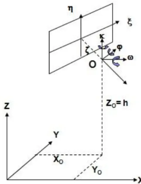
To handle mathematically the central projection defined by the images we need equations to describe the connection between the image points and the corresponding terrain points. To gain this purpose we basically use two important coordinate systems in photogrammetry. The first one is the image coordinate system (ξηζ), the second one is the (XYZ) terrain coordinate system (Figure 5-2).

Figure 5-2 Basic coordinate systems Notation: O: projection center,

ζ= : camera constant (calibrated focal length), ξηζ: image coordinate system,

XYZ: terrain coordinate system.

The image coordinate system is defined by the fiducial marks. These fiducial marks are located generally at the rim of the image in the corners or in the middle section of the image sides. The origin of the image coordinate system can be defined as the intersection point of lines gained by the opposite fiducial marks (Figure 5-3). The axis ζ of the image coordinate system is defined by the camera axis and each image coordinate ζ is a constant value and it is equal with the calibrated focal length called camera constant.

Figure 5-3 Image coordinate system

2.2. 5.2.2 Orientation Elements

(7)

If we want to evaluate the images and gain terrain coordinates we need to know the position of the image in the moment of exposure, it means we need to know the orientation elements. These elements can be divided into two groups: interior orientation elements and exterior orientation elements.

Interior orientation elements (Figures 5-2 and 5-3) are

• the image coordinates of the principal point ( , ),

• camera constant or focal length ( ).

The principal point is the point where the camera axis goes through the image plane virtually. This intersection point doesn’t fit with the intersection point of lines defined by the fiducial marks. Because of this, the coordinates of the principal point ( , ) should be considered at the central projection and in genera it is not equal zero.

Figure 5-2 also illustrates the exterior orientation elements. These elements are:

• geodetic coordinates of the perspective centre ( ),

• rotation angles defining the image plain orientation ( ).

The interior orientation elements are usually known with high accuracy, since these elements are defined in laboratory and supplemented to the camera. The exterior orientation elements should be defined during the aerial survey or after the exposure with calculation (for example with space resection method).

2.3. 5.2.3 Space Resection

The space resection can be solved using the collinear equations.

Equation 5-1 Collinear equations Notation:

: image coordinates,

: terrain coordinates,

: coordinates of the perspective centre,

: element of the rotation matrix, where each ,

: focal length.

The task is to determine the exterior orientation elements ( and ). Using the image and geodetic coordinates of at least four control points, we can solve the task with adjustment. First we need to linearize the Eq. 5-1 converting it to a Taylor polynomial. It means we have to generate partial derivatives by each unknown (exterior orientation element) and after that we can compile the error equations like:

(8)

Equation 5-2 Error equations of the space resection Notation:

a partial derivative gained from Eq. 5-1,

: corrections to the approximate values of unknowns,

: differences gained from the calculated and measured image coordinates,

: errors.

Also we need to determine the approximate values of unknowns as . Writing these approximations and the geodetic coordinates into the Eq. 5-1 we can get the calculated image coordinates as . If we decrement these values from the measured image coordinates, we can get the values (see Eq. 5-2).

The error equations Eq. 5-2 can be written into a matrix equation as .

The vector gives the corrections to the approximate values of unknowns. After making these corrections we repeat the whole procedure, and we continue it until the corrections become negligible. As a final result we gain the adjusted values of all exterior orientation elements.

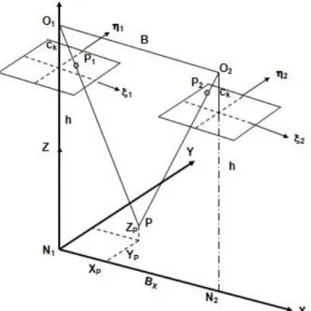
If we solve the task of space resection for one stereo-pair we can intersect the image rays to calculate the ground coordinates of any point (Figure 5-4).

Figure 5-4 Intersection of rays for calculation of the ground coordinates of P After the basics of coordinate systems, let’s list the data acquisition procedure based on images:

• Production of images.

(9)

• Orientation procedure, the reason of this step is to define the position of the images in the moment of exposure concerning the ground coordinate system.

• Photogrammetric evaluation and compilation of products like:

• Construction of a DTM model,

• Monoplotting,

• Orthophoto production,

• Mapping,

• Aerial triangulation,

• 3D modeling.

3. 5.3 Orientation Procedure

Before the evaluation, the orientation of images should be carried out. This procedure is usually done in three steps.

1. Interior orientation

Goal: To calculate the transformation parameters between the pixel and image coordinate systems.

For calculation of orientation elements (transformation parameters) we usually use the affine transformation:

Equation 5-3 Affine transformation Notation:

: image coordinates,

: pixel coordinates,

: affine parameters.

If we want to solve the transformation with adjustment we need to measure at least four fiducial marks.

2. Relative orientation

During the relative orientation we calculate the position of images in the 3D space. The position of images is calculated only relatively to each other and not to the global reference (or absolute) system. During the relative orientation the only condition is to position the image rays in such a position where they are intersecting each other, in other words the vectors should be in on plane. We call it as the co-planarity condition (Figure 5-5).

The relative position of two images can be described with 5 angle elements as .

(10)

Figure 5-5 Co-planarity condition And the co-planarity condition is:

Equation 5-4 Co-planarity condition Notation:

: Vector components of the basis . Usually we choose the model coordinate system with the origin of and the axis is parallel to the basis, which means, the and .

Model coordinates of image points, these are the coordinates of the end of vectors respectively.

To solve the Equation 5-4 with an adjustment procedure we need at least 6 model points to be measured.

3. Absolute orientation

The task is to transform the model into the mapping (or geodetic) coordinate system. This task is solved with a spatial similarity transformation:

Equation 5-5 Spatial similarity transformation Notation:

: Geodetic coordinates

: Model coordinates

: Scale factor

: Rotation matrix

The elements of the absolute orientation:

: Difference or shift elements,

: Rotation angles, (these angles are included in the rotation matrix),

(11)

: Scale factor.

4. 5.4 Photogrammetric Workstations

4.1. 5.4.1 Hardware Components

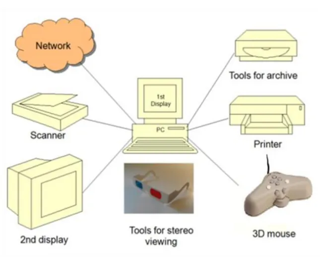
Basically the system is built on a computer with its display. The other tools are connected to the PC. (Figure 5- 6).

Figure 5-6 Elements of a digital photogrammetric workstation

The PC as a central element of the system is a high category personal computer. Especially the capacity of the RAM and the hard disk are very important because of the processing of digital images.

The requirements towards the video card depend on the tools used for stereo viewing. You can read more details in chapter 5.4.2.

The evaluation process can be faster and more comfortable if we can use two displays. The secondary display is usually used for file browsing and other displaying of text information, or it helps in the stereo viewing splitting the images of the stereo-pair to left and right images.

If we have only analogue images then we need to scan them using office or professional photogrammetric scanners.

The goal of the network connection is to have access to archiving computers, or we can distribute the results for further processing over the network. The network connection makes also possible to organize a team-work over a certain project, where the images can be stored on a central server, which can be reached by each user. This approach facilitates also the controlling of the work and the actual state of the project.

After completing the evaluation, the printers and plotters are used to print or draw out the results.

(12)

For measuring the coordinates on the images we need a 3D mouse (sometimes it is called as hand-held cursor).

If we don’t have a special mouse dedicated for photogrammetric measurement, then we can use a simple PC mouse having a track-wheel. During the measurements we can face other tasks like rotating, moving or zooming of images. Therefore it is wise to have a 3D mouse, which has extra buttons to make these functions available (Figure 5-7).

Figure 5-7 3D mice developed for photogrammetric evaluation

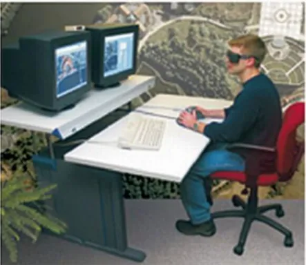
Figure 5-8 shows a digital photogrammetric workstation as an example. Looking at the photo we can discover the system elements:

Figure 5-8 Example of a photogrammetric workstation

4.2. 5.4.2 Stereo Viewing Methods

On digital photogrammetric workstations basically four different methods are used for stereo viewing.

These methods are the following:

• Anaglyph viewing,

• Stereo viewing with split display,

• Stereo viewing with flickering images using an active polarization,

(13)

• Stereo viewing with passive polarization.

Each viewing method has a tool or equipment facilitating the stereo viewing on the computer display.

Let’s overview each method:

Anaglyph viewing

The anaglyph stereo viewing is based on color filtering. The viewing tool is a pair of eye-glasses having red and blue color filters. The images of the stereo-pair are displayed on the monitor in red and blue (or in red and green) colors. The function of the eye-glasses is the filtering. Each side is transparent only to its complementary color, which means that the red filter transfers only the blue color, the blue filter is transparent only for the red color. By this simple method we can assure the stereo effect. Color images can be used only with restriction, since only the red and the blue colors make the parallax effect (Figure 5-9).

Figure 5-9 Anaglyph image Stereo viewing with split display

At this method the display area is split, and the left and right image of the stereo-pair is displayed side by side.

For viewing we need a mirror stereoscope, which is fixed to the monitor with a steel arm (Figure 5-11). Through the stereoscope each eye can see only the appropriate image, which is overlapped in our brain forming a stereo model.

Stereo viewing with flickering images

Using this active polarization method we need a video card having the capability to display the images in stereo flickering mode, which means that the left and the right images are displayed separately after each other following the monitor frequency. For example, if we have a 100 Hertz monitor, then the left and the right images are flickered 50 times in one second. For viewing these images we need a pair of eye-glasses having an

(14)

active polarization operating by liquid crystal technology. Here the polarization means that in one moment only one side is transparent, the other side is black. This polarization is made in harmony with the monitor frequency.

To reach the polarization, the eye-glasses are connected to the video card with a wire. The connection can be wireless, but in this case we need an infra emitter connected to the video card. This infra emitter controls the polarization (flickering) of the eye-glasses (Figure 5-10).

Figure 5-10 Liquid crystal eye-glasses and the infra emitter Stereo viewing with passive polarization

Following this method, a polarization glass-panel – so called Z-screen - is attached to the display. Through this filter only vertical and horizontal rays can leave the monitor (Figure 5-11). The images of the stereo-pair are displayed separately after each other and the Z-screen polarizes these images. For separation of the images we need passive eye-glasses having horizontal and vertical ray filters. As a result we see the images with the appropriate eye, the left image with the left eye, the right image with the right eye.

Figure 5-11 Z-screen

The other technique of the passive polarization is when we have two monitors and between them we have a polarization panel as a half-mirror. The first display is opposite to us; the other one is inclined and located above the other monitor. A half-transparent panel is fixed between the monitors, in the same time this panel polarizes the images. The panel transfers the opposite image (this is the left image of the stereo-pair) only with horizontal rays, the right image coming from the upper monitor is reflected only by vertically rays. The pair of passive polarization eye-glasses assures the separation of horizontal and vertical rays (Figure 5-12).

(15)

Figure 5-12 3D viewing with a system having two displays and a polarization panel

5. 5.5 Evaluation Software Modules

The digital photogrammetric workstations offer a wide range of evaluation and processing software. We cannot list all of them, but we can find common software modules by function among the different workstations. In the following chapters we try to describe them.

5.1. 5.5.1 Scanner Calibration

The goal of the scanner calibration is to determine the systematic errors. For investigation a calibration grid is used, which is scanned by the scanner. The coordinates of the grid points are known with high accuracy. After scanning the grid, the coordinates of the grid points are measured on the scanned image of the calibration grid.

Using affine or other polynomial transformation we can compare the original grid coordinates with the scanned grid coordinates and we can determine the systematic errors at each grid point. The measurement of the scanned grid point can be automatic if the evaluation software is able to use some image matching algorithm. (Figure 5- 13).

Figure 5-13 Grid measurement on a photogrammetric workstation

The calculated systematic errors and the transformation parameters are stored in a calibration file. Using this file later the coordinates of image points can be corrected.

(16)

5.2. 5.5.2 Orientation of Images

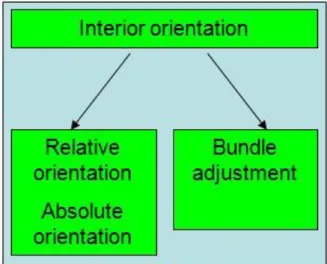
On the photogrammetric workstation it is possible to make the orientation of one image, an image pair or even a block of images. The orientation of one image can be done by space resection using the equations 5-1. On Figure 5-14 we can see that the orientation procedure can be done by two different ways. Among the ways the common step is the interior orientation. The two different exterior orientation procedures are:

1. Relative and absolute orientation,

2. Bundle adjustment. This adjustment procedure is based on the Eg. 5-1, where the space resection and intersection tasks are solved simultaneously using all the bundle of image rays.

Figure 5-14 Hierarchy of the orientation procedure

Basic mathematical principles of these two orientation procedures are explained by Equations 5-1, 5-2, 5-3 and 5-4. The measurement of the points necessary for the interior and relative orientation can be automatic, for this purpose usually Equation 5-5 is used to carry out an area-based image matching algorithm.

5.3. 5.5.3 Digital Terrain Modeling

Using a stereo-pair, the DTM data acquisition can be an automatic process using different stereo-correlation methods.

Among the correlation methods a common point is to find the homolog point pairs (the same terrain point on the overlapping area of a stereo-pair). To reach this goal, sample areas (correlation matrices) are compared. The search can be extended to lines and other complex figures, but usually the area-based matching is carried out to find common points.

The Equation 5-6 shows the most frequently used cross-correlation equation (Höhle 2003):

Equation 5-6 Cross-correlation Notation:

- grey value inside the target (left image) sample,

- grey value inside the search area (fragment of the right image),

- row, column index,

(17)

- mean value calculated from the grey values on the target and the search areas,

- number of rows and columns of the sample area.

The autocorrelation process is not fully exact; therefore the gained DTM should be checked and corrected by the operator. To help the operator’s work, a correlation image can be produced showing the weakly correlated areas (Figure 5-15).

Figure 5-15 Checking of the DTM on a Leica LPS workstation

5.4. 5.5.4 Monoplotting

Monoplotting as an evaluation method is based only on single images. The main idea is to gain X, Y, Z coordinates using the image and an associated DTM model. Also we need to know the interior and exterior orientation elements. The X, Y coordinates are calculated by the image point with the help of Equation 5-1, the Z coordinate is interpolated from the DTM (Figure 5-16). The measurement of the terrain coordinates can be continuous and the drawing lines and other mapping features can be organized in real-time regime.

(18)

Figure 5-16 Principle of the monoplotting evaluation method

5.5. 5.5.5 Creation of Digital Orthophotos

The digital orthophoto is gained from the original photo. During the ortho- rectification we eliminate the perspective and height distortions at each image point. The reason of perspective distortion is that the image plane and the terrain is not parallel, the height distortion is caused by the differences in height on the terrain.

After eliminating these distortions the resulted image, the orthophoto can be used for mapping purposes directly.

We can print it out in a certain scale; we can draw on it all the content which usually can be seen on a normal cartographic map.

For elimination of these distortions we need to know the orientation elements and the DTM covering the image area.

If the target area is larger than one photo, we need to produce an orthophoto mosaic image. From this mosaic an orthophoto map is produced, when we add to it the coordinate grid, the scale and other necessary mapping elements.

This procedure is summarized on Figure 5-17 (Aranoff 1995).

(19)

Figure 5-17 Process of the orthophoto production

To produce the orthophoto we need Equation 5-1. First we generate an X, Y coordinate system as a pixel coordinate system of the orthophoto on the mapping projection plane. It means we bind an X, Y coordinate to each pixel of the orthophoto with step of dX, dY (see Figure 5-19). After this the defined image pixels are transformed back to image plane defined in the camera coordinate system using Equation 5-1. For this we need to know also the interior orientation elements ( ) and exterior orientation elements (

) (Albertz J., Kreiling W. (1989)).

All this procedure can be more understandable examining Figure 5-18 (Kraus 1998).

(20)

Figure 5-18 Connection between the grid defined on X, Y plane and the distorted grid on the image During the pixel transformation (resampling) we face two problems (Kraus 1998):

1. It is possible, that during the transformation there will be pixels on the original image where the transformed point is missing, it means these pixels disappear from the original image and cannot be visible in the produced orthophoto.

Solution: The number of pixels should be incremented on the orthophoto. If the terrain is not hilly, 25%

increment in number of pixels is enough. If the terrain is a hilly area then the number of pixels can be doubled.

2. The transformed pixel will not cover exactly the pixel of the original image (Figure 5-19) therefore we have to decide somehow a new grey value to the transformed pixel.

(21)

Figure 5-19 Transformation of the orthophoto image matrix into the original image matrix

This procedure is called resampling and it can be solved by the following ways:

• Let’s choose the closest neighboring pixel and its grey value will be inherited. This simple method can cause one pixel shift, which is more visible along line features (like roads) in the orthophoto.

• We can gain visually a smoother result, if we use the four neighboring pixels and theirs grey value of the pixel width is . For calculation of the grey value of the transformed pixel we use a bilinear interpolation using Equation 5-6 (Kraus-Waldhäusl 1998):

Figure 5-7 Bilinear interpolation

• We can raise the accuracy if we take more neighboring points, for example 16 points, but the calculation time will be much more.

5.6. 5.5.6 Mapping

The mapping procedure is organized by one image or by image pairs. If we prefer the mapping based on single images, we can choose the monoplotting method or we can take directly the produced orthophoto.

When we use an image-pair we have a possibility for 3D mapping after completing the orientation procedure (interior and exterior orientation). We can use the general CAD mapping software for the evaluation, but in this case we will need an interface program, which connects the photogrammetric software with the mapping application. The other choice is to use the built-in mapping software inside the workstation environment.

Usually the built-in mapping software is simpler than the professional CAD applications like AutoCad or Microstation (Figure 5-21). This approach is shown on Figure 5-20.

(22)

Figure 5-20 Different approaches to the mapping procedure applied in digital photogrammetry

Figure 5-21 Mapping in Microstation environment

5.7. 5.5.7 Aerial Triangulation

The goal of the aerial triangulation is to calculate the exterior orientation elements of all images connected together in one block. Also we have to calculate the coordinates of new points which will serve as control points or tie points between the images (Figure 5-22); these points are found on the overlapping areas of three or more images.

(23)

We need to measure the existed control points to fit the whole block into the geodetic coordinate system, the new points and the tie points. The tie points are necessary to tie the overlapping images and they can be measured automatically with an auto-correlation method.

Figure 5-22 Aerial triangulation block on a DVP workstation

Usually the aerial triangulation software is an independent application and it is able to receive data from different workstations. The program uses different methods for gaining the goal. Recent aerial triangulation software packages use both methods, the block adjustment of independent models and bundle adjustment procedure based on image coordinates. The weak point of the bundle adjustment is that it needs initial values of the unknown orientation elements to solve all equations of 5-1 at each image ray. To calculate the necessary initial values, the triangulation software uses the results of the block adjustment based on independent models.

Other alternative is to form first models, then from the models we form rows and from the rows a block is generated. Following this strategy we can find and eliminate the gross errors in an easier way. The final procedure is the bundle adjustment, where each image ray is participating in the adjustment procedure (Figure 5- 23).

(24)

Figure 5-23 Procedure of the aerial triangulation

5.8. 5.5.8 3D modeling

It is a special case at the photogrammetric evaluation and mapping when we produce 3D mapping objects instead of the usual 2D map features. The most developed systems are capable to organize the 3D mapping objects in an object oriented way as it is more common at other information sciences or programming languages. We need to build a database of 3D objects, where the objects are connected to each other by object oriented logic (like inheritance, polymorphism, hierarchy, etc.). Not every photogrammetric system meets this requirement. Usually the only requirement is to produce the 3D model as a unique object and the images are rendered on this model to produce a photorealistic 3D model.

The generated models can be used on different areas; a typical example is Google Earth, where the users can produce 3D models using the tools offered by the company Google (Figure 5-24).

Figure 5-24 Example of a city model in Google Earth environment Some typical areas for using of 3D models are:

• Urban planning, architecture (Figure 5-25),

• Archeology,

• Civil engineering,

• Industrial design and reverse engineering.

(25)

Figure 5-25 Simplified 3D models of buildings and city districts

6. 5.6 Summary

In this module we introduced the basics of photogrammetry, especially the digital photogrammetry. We listed the possible products and evaluation procedures of the digital photogrammetric workstations (DPW). We divided the module into two logical parts. The first part explains the basic mathematical principles of the photogrammetric orientation and evaluation. The second part gives an overview about the DPWs and the products gained by them.

Questions for self-test:

1. How can you structure photogrammetry? /page 4/

2. What are the interior and exterior orientation elements? /page 6/

3. Explain the orientation procedure. /pages 9-11 and 19/

4. Explain the parts of a digital photogrammetric workstation. /page 12/

5. Explain the principle of the stereo viewing system using a passive polarization technique with two LCDs.

/page 17/

6. During the image orientation which points can be measured automatically? /page 19/

7. How can be the DTM production an automatic process? /page 20/

8. What kind of data do we need to know during the digital monoplotting? /page 21/

9. What is the most important equation during the orthophoto production? /page 22/

10. During the mapping how can you connect AutoCad to the photogrammetric software? /page 25/

11. What is the final adjustment procedure at the aerial triangulation? /page 27/

(26)

12. What are the typical areas of using the 3D models? (page 29/

References:

1. Aranoff, S. : Geographic Information Systems: A management perspective, WDL Publications, Ottawa, Canada, 1995

2. Albertz J., - Kreiling W. : Photogrammetrisches Taschenbuch, Herbert Wichmann Verlag, 1989

3. Ebner H., Fritsch D., Heipke C. (szerk.) (1991): Digital photogrammetric systems, Herbert Wichmann Verlag GmbH, Karlsruhe, 1991

4. Ecker R., Kalliany R., Gottfried O. : High quality rectification and image enhancement techniques for digital orthophoto producton, Photogrammetric Week’93, Herbert Wichmann Verlag GmbH, Karlsruhe, 1993

4. Höhle, J. - Potucková M.: Automated quality control for orthoimages and DEMS, Aalborg University, Aalborg, 2003

6. Kraus K. : Photogrammetry, Walter de Gruyter, Berlin, 2007