Artificial Intelligence

(1)

Artificial Intelligence

Gergely Kovásznai

Gábor Kusper

(2)

Artificial Intelligence

Gergely Kovásznai Gábor Kusper Publication date 2011

(3)

Chapter 1. Introduction

Surely everyone have thought about what artificial intelligence is? In most cases, the answer from a mathematically educated colleague comes in an instant: It depends on what the definition is? If artificial intelligence is when the computer beats us in chess, then we are very close to attain artificial intelligence. If the definition is to drive a land rover through a desert from point A to point B, then we are again on the right track to execute artificial intelligence. However, if our expectation is that the computer should understand what we say, then we are far away from it.

This lecture note uses artificial intelligence in the first sense. We will bring out such „clever” algorithms, that can be used to solve the so called graph searching problems. The problems that can be rewritten into a graph search – such as chess – can be solved by the computer.

Alas, the computer will not become clever in the ordinary meaning of the word if we implement these algorithms, at best, it will be able to systematically examine a graph in search of a solution. So our computer remains as thick as two short planks, but we exploit the no more than two good qualities that a computer has, which are:

1. The computer can do algebraic operations (addition, subtraction, etc.) very fast.

2. It does these correctly.

So we exploit the fact that such problems that are to difficult for a human to see through – like the solution of the Rubik Cube – are represented in graphs, which are relatively small compared to the capabilities of a computer, so quickly and correctly applying the steps dictated by the graph search algorithms will result in a fast-solved Cube and due to the correctness, we can be sure that the solution is right.

At the same time, we can easily find a problem that's graph representation is so huge, that even the fastest computers are unable to quickly find a solution in the enormous graph. This is where the main point of our note comes in: the human creativity required by the artificial intelligence. To represent a problem in a way that it's graph would keep small. This is the task that should be started developing in high school. This requires the expansion of the following skills:

1. Model creation by the abstraction of the reality 2. System approach

It would be worthwhile to add algorithmic thinking to the list above, which is required to think over and execute the algorithms published in this note. We will talk about this in a subsequent chapter.

The solution of a problem is the following in the case of applying artificial intelligence:

1. We model the real problem.

2. We solve the modelled problem.

3. With the help of the solution found in the model, we solve the real problem.

All steps are helped by different branches of science. At the first step, the help comes from the sciences that describe reality: physics, chemistry, etc. The second step uses an abstract idea system, where mathematics and logic helps to work on the abstract objects. At last, the engineering sciences, informatics helps to plant the model's solution into reality.

This is all nice, but why can't we solve the existing problem in reality at once? Why do we need modelling? The answer is simple. Searching can be quite difficult and expensive in reality. If the well-know 8 Queens Problem should be played with 1-ton iron queens, we would also need a massive hoisting crane, and the searching would take a few days and a few hundreds of diesel oil till we find a solution. It is easier and cheaper to search for a solution in an abstract space. That is why we need modelling.

(6)

Introduction

What guarantees that the solution found in the abstract space will work in reality? So, what guarantees that a house built this way will not collapse? This is a difficult question. For the answer, let's see the different steps in detail.

Modelling the existing problem:

1. We magnify the parts of the problem that are important for the solution and neglect the ones that are not.

2. We have to count and measure the important parts.

3. We need to identify the possible „operators” that can be used to change reality.

Modelling the existing problem is called state space representation in artificial intelligence. We have a separate chapter on this topic. We are dealing with this question in connection with the „will-the-house-collapse” - issue.

Unfortunately, a house can be ruined at this point, because if we neglect an important issue, like the depth of the wall, the house may collapse. How does this problem, finding the important parts in a text, appear in secondary school? Fortunately, it's usually a maths exercise, which rarely contains unnecessary informations. The writer of the exercise usually takes it the other way round and we need to find some additional information which is hidden in the text.

It is also important to know that measuring reality is always disturbed with errors. With the tools of Numeric mathematics, the addition of the the initial errors can be given, so the solution's error content can also be given.

The third step, the identification of the „operators”, is the most important in the artificial intelligence's aspect.

The operator is a thing, that changes the part of reality that is important for us, namely, it takes from one well- describable state into another. Regarding artificial intelligence, it's an operator, when we move in chess, but it may not if we chop down a tree unless the number of the trees is not an important detail in the solution of the problem.

We will see that our model, also know as state space can be given with 1. the initial state,

2. the set of end states, 3. the possible states and

4. the operators (including the pre and post condition of the operators).

We need to go through the following steps to solve the modelled problem:

1. Chose a framework that can solve the problem.

2. Set the model in the framework.

3. The framework solves the problem.

Choosing the framework that is able to solve our model means choosing the algorithm that can solve the modelled problem. This doesn't mean that we have to implement this algorithm. For example, the Prolog interpreter uses backtrack search. We only need to implement, which is the second step, the rules that describe the model in Prolog. Unfortunately, this step is influenced by the fact, that we either took transformational- (that creates a state from another state) or problem reduction (that creates more states from another state) operators in the state space representation. So we can take the definition of the operators to be the next step after choosing the framework. The frameworks may differ from each other in many ways, the possible groupings are:

1. Algorithms, that surly find the solution in a limited, non-circle graph.

2. Algorithms, that surly find the solution in a limited graph.

3. Algorithms, that give an optimal solution according to some point of view.

If we have the adequate framework, our last task is to implement the model in the framework. This is usually means setting the initial state, the end condition and the operators (with pre- and postconditions). We only need

(7)

to push the button, and the framework will solve the problem if it is able to do it. Now, assume that we have got a solution. First of all, we need to know what do we mean under 'solution'. Solution is a sequence of steps (operator applications), that leads from the initial state into an end state. So, if the initial state is that we have enough material to build a house and the end state is that a house had been built according to the design, then the solution is a sequence of steps about how to build the house.

There is only one question left: will the house collapse? The answer is definitely 'NO', if we haven't done any mistake at the previous step, which was creating the model, and will not do at the next step, which is replanting the abstract model into reality. The warranty for this is the fact that the algorithms introduced in the notes are correct, namely by logical methods it can be proven that if they result in a solution, that is a correct solution inside the model. Of course, we can mess up the implementation of the model (by giving an incorrect end condition, for example), but if we manage to evade this tumbler, we can trust our solution in the same extent as we can trust in logics.

The last step is to solve the real problem with the solution that we found in the model. We have no other task than executing the steps of the model's solution in reality. Here, we can face that a step, that was quite simple in the model (like move the queen to the A1 field) is difficult if not impossible in reality. If we found that the step is impossible, than our model is incorrect. If we don't trust in the solution given by the model, then it worth trying it in small. If we haven't messed up neither of the steps, then the house will stand, which is guaranteed by the correctness of the algorithms and the fact that logic is based on reality!

(8)

Chapter 2. The History of Artificial Intelligence

Studying the intelligence is one of the most ancient scientific discipline. Philosopher have been trying to understand for more than 2000 years what mechanism we use to sense, learn, remember, and think. From the 2000 years old philosophical tradition the theory of reasoning and learning have developed, along with the view that the mind is created by the functioning of some physical system. Among others, these philosophical theories made the formal theory of logic, probability, decision-making, and calculation develop from mathematics..

The scientific analysis of skills in connection with intelligence was turned into real theory and practice with the appearance of computers in the 1950s. Many thought that these „electrical masterminds” have infinite potencies regarding executing intelligence. „Faster than Einstein” - became a typical newspaper article. In the meantime, modelling intelligent thinking and behaving with computers proved much more difficult than many have

thought at the beginning.

(9)

Figure 1. The early optimism of the 1950s: „The smallest electronic mind of the world” :)

The Artificial Intelligence (AI) deals with the ultimate challenge: How can a (either biological or electronic) mind sense, understand, foretell, and manipulate a world that is much larger and more complex than itself? And what if we would like to construct something with such capabilities?

AI is one of the newest field of science. Formally it was created in 1956, when its name was created, although some researches had already been going on for 5 years. AI's history can be broken down into three major periods.

(10)

The History of Artificial Intelligence

1. Early Enthusiasm, Great Expectations (Till the end of the 1960s)

In a way, the early years of AI were full of successes. If we consider the primitive computers and programming tools of that age, and the fact, that even a few years before, computers were only though to be capable of doing arithmetical tasks, it was astonishing to think that the computer is – even if far from it – capable of doing clever things.

In this era, the researchers drew up ambitious plans (world champion chess software, universal translator machine) and the main direction of research was to write up general problem solving methods. Allen Newell and Herbert Simon created a general problem solving application (General Program Solver, GPS), which may have been the first software to imitate the protocols of human-like problem solving.

This was the era when the first theorem provers came into existence. One of these was Herbert Gelernter's Geometry Theorem Prover, which proved theorems based on explicitly represented axioms.

Arthur Samuel wrote an application that played Draughts and whose game power level reached the level of the competitors. Samuel endowed his software with the ability of learning. The application played as a starter level player, but it became a strong opponent after playing a few days with itself, eventually becoming a worthy opponent on strong human race. Samuel managed to confute the fact that a computer is only capable of doing what it was told to do, as his application quickly learnt to play better than Samuel himself.

In 1958, John McCarthy created theLisp programming language, which outgrew into the primary language of AI programming. Lisp is the second oldest programming language still in use today.

2. Disillusionment and the knowledge-based systems (till the end of the 1980s)

The general-purpose softwares of the early period of AI were only able to solve simple tasks effectively and failed miserably when they should be used in a wider range or on more difficult tasks. One of the sources of difficulty was that early softwares had very few or no knowledge about the problems they handled, and achieved successes by simple syntactic manipulations. There is a typical story in connection with the early computer translations. After the Sputnik's launch in 1957, the translations of Russian scientific articles were hasted. At the beginning, it was thought that simple syntactic transformations based on the English and Russian grammar and word substitution will be enough to define the precise meaning of a sentence. According to the anecdote, when the famous „The spirit is willing, but the flesh is weak” sentence was re-translated, it gave the following text:

„The vodka is strong, but the meat is rotten.” This clearly showed the experienced difficulties, and the fact that general knowledge about a topic is necessary to resolve the ambiguities.

The other difficulty was that many problems that were tried to solve by the AI were untreatable. The early AI softwares were trying step sequences based on the basic facts about the problem that should be solved, experimented with different step combinations till they found a solution. The early softwares were usable because the worlds they handled contained only a few objects. In computational complexity theory, before defining NP-completeness (Steven Cook, 1971; Richard Karp, 1972), it was thought that using these softwares for more complex problems is just matter of faster hardware and more memory. This was confuted in theory by the results in connection with NP-completeness. In the early era, AI was unable to beat the „combinatorial boom” – combinatorial explosion and the outcome was the stopping of AI research in many places.

From the end of the 1960s, developing the so-called expert systems were emphasised. These systems had (rule- based) knowledge base about the field they handled, on which an inference engine is executing deductive steps.

In this period, serious accomplishments were born in the theory of resolution theorem proving (J. A. Robinson, 1965), mapping out knowledge representation techniques, and on the field of heuristic search and methods for handling uncertainty. The first expert systems were born on the field of medical diagnostics. The MYCIN system, for example, with its 450 rules, reached the effectiveness of human experts, and put up a significantly better show than novice physicians.

At the beginning of the 1970s, Prolog, the logical programming language were born, which was built on the computerized realization of a version of the resolution calculus. Prolog is a remarkably prevalent tool in

(11)

developing expert systems (on medical, judiciary, and other scopes), but natural language parsers were implemented in this language, too. Some of the great achievements of this era is linked to the natural language parsers of which many were used as database-interfaces.

3. AI becomes industry (since 1980)

The first successful expert system, called R1, helped to configure computer systems, and by 1986, it made a 40 million dollar yearly saving for the developer company, DEC. In 1988, DEC's AI-group already put on 40 expert systems and was working on even more.

In 1981, the Japanese announced the „fifth generation computer” project – a 10-year plan to build an intelligent computer system that uses the Prolog language as a machine code. Answering the Japanese challenge, the USA and the leading countries of Europe also started long-term projects with similar goals. This period brought the brake-through, when the AI stepped out of the laboratories and the pragmatic usage of AI has begun. On many fields (medical diagnostics, chemistry, geology, industrial process control, robotics, etc.) expert systems were used and these were used through a natural language interface. All in all, by 1988, the yearly income of the AI industry increased to 2 billion dollars.

Besides expert systems, new and long-forgotten technologies have appeared. A big class of these techniques includes statistical AI-methods, whose research got a boost in the early years of the 1980's from the (re)discovery of neural networks. The hidden Markov-models, which are used in speech- and handwriting- recognition, also fall into this category. There had been a mild revolution on the fields of robotics, machine vision, and learning.

Today, AI-technologies are very versatile: they mostly appear in the industry, but they also gain ground in everyday services. They are becoming part of our everyday life.

(12)

Chapter 3. Problem Representation

1. State-space representation

The first question is, how to represent a problem that should be solved on computer. After developing the details of a representation technology, we can create algorithms that work on these kind of representations. In the followings, we will learn the state-space representation, which is a quite universal representation technology.

Furthermore, many problem solving algorithms are known in connection with state-space representation, which we will be review deeply in the 3rd chapter.

To represent a problem, we need to find a limited number of features and parameters (colour, weight, size, price, position, etc.) in connection with the problem that we think to be useful during the solving. For example, if these parameters are described with the values (colour: black/white/red; temperature: [-20C˚, 40C˚]; etc.), then we say that the problem's world is in thestate identified by the vector . If we denote the set which consists of values adopted by the i. parameter with Hi , then the states of the problem's world are elements

of the set .

As we've determined the possible states of the problem's word this way, we have to give a special state that specifies the initial values of the parameters in connection with the problem's world. This is called the initial state.

Now we only need to specify which states can be changed and what states will these changes call forth. The functions that describe the state-changes are called operators. Naturally, an operator can't be applied to each and every state, so the domain of the operators (as functions) is given with the help of the so-called preconditions.

Definition 1. A state-space representation is a tuple , where:

1. A: is the set of states, A ≠ ࢝, 2. k ∈A: is the initial state, 3. C ⊆A: is the set of goal states, 4. O: is the set of the operators, O ≠ ࢝.

Every o∈O operator is a function o: Dom(o)→A, where

(3.1)

The set C can be defined in two ways:

• By enumeration (in an explicit way):

• By formalizing a goal condition (in an implicit way):

The conditions preconditiono(a) and goal condition(a) can be specified as logical formulas. Each formulas' parameter is a state a, and the precondition of the operator also has the applicable operator o.

Henceforth, we need to define what we mean the solution of a state-space represented problem – as that is the thing we want to create an algorithm for. The concept of a problem's solution can be described through the following definitions:

Definition 2. Let be a state-space representation, and a, a' ∈A are two states.

a' is directly accessible from a if there is an operator o ∈O where preconditiono(a) holds and o(a)=a'.

(13)

Notation: .

Definition 3. Let be a state-space representation, and a, a' ∈A are two states.

a' is accessible from a if there is a a1, a2, ..., an state sequence where

• ai=a,

• an=a'

• : (any operator) Notation:

Definition 4.The problem is solvable if for any goal state . In this case, the operator sequence is referred as a solution to the problem.

Some problems may have more than one solution. In such cases, it can be interesting to compare the solutions by their costs - and select the less costly (the cheapest) solution. We have the option to assign a cost to the application of an operator to the state a, and denote it as costo(a) (assuming that o is applicable to a, that is, preconditiono(a) holds), which is a positive integer.

Definition 5. Let in the case of a problem for any . The cost of the solution is:

(3.2)

Namely, the cost of a solution is the cost of all the operator applications in the solution. In the case of many problems, the cost of operator applications is uniform, that is cost(o,a)=1 for any operator o and state a. In this case, the cost of the solution is implicitly the number of applied operators.

2. State-space graph

The best tool to demonstrate the state-space representation of a problem is the state-space graph.

Definition 6. Let be the state-space representation of a problem. The problem's state-space graph is the graph¹ , where (a,a')∈E and (a, a') is labelled with o if and only if .

Therefore, the vertices of the state-space graph are the states themselves, and we draw an edge between two vertices if and only if one vertex (as a state) is directly accessible from another vertex (as a state). We label the edges with the operator that allows the direct accessibility.

It can be easily seen that a solution of a problem is nothing else but a path that leads from a vertex k (aka the initial vertex) to some vertex c∈C (aka the goal vertex). Precisely, the solution is the sequence of labels (operators) of the edges that formulate this path.

In Chapter 4, we will get to know a handful of problem solving algorithms. It can be said, in general, that all of them explore the state-space graph of the given task in different degree and look for the path that represents the solution in the graph.

3. Examples

1As usual: is the set of the graph's vertices, is the set of the graph's edges.

(14)

Problem Representation

In this chapter, we introduce the possible state-space representations of several noteworthy problems.

3.1. 3 Jugs

We have 3 jugs of capacities 3, 5, and 8 litres, respectively. There is no scale on the jugs, so it's only their capacities that we certainly know. Initially, the 8-litre jug is full of water, the other two are empty:

We can pour water from one jug to another, and the goal is to have exactly 4 litres of water in any of the jugs.

The amount of water in the other two jugs at the end is irrelevant. Here are two of the possible goal states:

Since there is no scale on the jugs and we don't have any other tools that would help, we can pour water from jug A to jug B in two different ways:

• We pour all the water from jug A to jug B.

• We fill up jug B (and it's possible that some water will remain in jug A).

Give a number to each jug: let the smallest be 1, the middle one 2, and the largest one 3! Generalize the task to jugs of any capacity: introduce a vector with 3 components (as a constant object out of the state-space), in which we store the capacities of the jugs:

(3.3)

• Set of states: In the states, we store the amount of water in the jugs. Let the state be an tuple, in which the i^th part tells about the jug denoted by i how many litres of water it is containing. So, the set of states is defined as follows:

(15)

where every ai is an integer.

• Initial state: at first, jug 3 is full all, the other ones are empty. So, the initial state is:

(3.4)

• Set of goal states: We have several goal states, so we define the set of goal states with help of a goal condition:

(3.5)

• Set of operators: Our operators realize the pouring from one jug (denoted by i) to another one (denoted by j).

We can also specify that the source jug (i) and the goal jug (j) can't be the same. Our operators are defined as follows:

(3.6)

• Precondition of the operators: Let's define when an operator pouri,j can be applied to a state (a1, a2, a3)! It's practical to specify the following conditions:

• Jug i is not empty.

• Jug j is not filled.

So, the precondition of the operator pouri,j to the state (a1, a2, a3) is:

(3.7)

• Function of applying: Define what state (a'1, a'2, a'3) does the operator pouri,j create from the state (a1, a2, a3)!

The question is how many litres of water can we pour from jug i to jug j. Since at most

(3.8)

litres of water can be poured to jug j, we can calculate the exact amount to be poured by calculating

(3.9)

Denote this amount with T. Consequently: pouri,j(a1, a2, a3)=(a'1, a'2, a'3), where

(3.10)

(3.11)

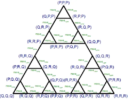
State-space graph. The state-space graph of the aforementioned state-space representation can be seen in Figure 2.

(16)

Figure 2. The state-space graph of the 3 Jugs problem.

In the graph, the red lines depict unidirectional edges while the green ones are bidirectional edges. Naturally, bidirectional edges should be represented as two unidirectional edges, but due to lack of space, let us use bidirectional edges. It can be seen that the labels of the bidirectional edges are given in the form of pouri, j1-j2 , which is different from the form of pouri, j as it was given in the state-space representation. The reason for this is that one pouri, j1-j2 label encodes two operators at the same time: the operators pouri, j1 and pouri, j2 .

The green vertices represent the goal states. The bold edges represent one of the solutions, which is the following operator sequence:

(3.12)

Notice that the problem has several solutions. It can also be noticed that the state-space graph contains cycles , that makes it even more difficult to find a solution.

3.2. Towers of Hanoi

There are 3 discs with different diameters. We can slide these discs onto 3 perpendicular rods. It's important that if there is a disc under another one then it must be bigger in diameter. We denote the rods with „P”, „Q”, and

„R”, respectively. The discs are denoted by „1”, „2”, and „3”, respectively, in ascending order of diameter. The initial state of discs can be seen in the figure below:

(17)

We can slide a disc onto another rod if the disc 1. is on the top of its current rod, and

2. the discs on the goal rod will be in ascending order by size after the replacing.

Our goal is to move all the discs to rod R.

We create the state-space representation of the problem, as follows:

• Set of states: In the states, we store the information about the currently positions (i.e., rods) of the discs. So, a state is a vector (a1, a2, a3) where ai is the position of disc i (i.e., either P, Q, or R). Namely:

(3.13)

• Initial state: Initially, all the discs are on rod P, i. e.:

(3.14)

• Set of goal states: The goal is to move all the three discs to rod R. So, in this problem, we have only one goal state, namely:

(3.15)

• Set of operators: Each operator includes two pieces of information:

• which disc to move

• to which rod?

Namely:

(3.16)

• Precondition of the operators: Take an operator movewhich, where ! Let's examine when we can apply it to a state (a1, a2, a3)! We need to formalize the following two conditions:

1. The disc which is on the top of the rod awhich .

2. The disc which is getting moved to the top of the rod where.

What we need to formalize as a logical formula is that each disc that is smaller than disc which (if such one does exist) is not on either rod awhich or rod where.

(18)

It's worth to extend the aforementioned condition with another one, namely that we don't want to move a disc to the same rod from which we are removing the disc. This condition is not obligatory, but can speed up the search (it will eliminate trivial cycles in the state-space graph). Thus, the precondition of the operators is:

(3.17)

• Function of applying: Take any operator movewhich, where ! If the precondition of the operator holds to a state (a1, a2, a3), then we can apply it to this state. We have to formalize that how the resulting state (a'1, a'2, a'3) will look like.

We have to formalize that the disc which will be moved to the rod where, while the other discs will stay where they currently are. Thus:

(3.18)

Important note: we have to define all of the components of the new state, not just the one that changes!

State-space graph. The state-space graph of the aforementioned state-space representation can be seen in Figure 3.

Figure 3. The state-space graph of the Towers of Hanoi problem.

Naturally, all of the edges in the graph are bidirectional, and their labels can be interpreted as in the previous chapter: a label movei, j1-j2 refers to both the operators movei, j1 and áti, j2 .

As it can be clearly seen in the figure, the optimal (shortest) solution of the problem is given by the rightmost side of the large triangle, namely, the optimal solution consists of 7 steps (operators).

3.3. 8 queens

Place 8 queens on a chessboard in a way that no two of them attack each other. One possible solution:

(19)

Generalize the task to a chessboard, on which we need to place N queens. N is given as a constant out of the state-space.

The basic idea of the state-space representation is the following: since we will place exactly one queen to each row of the board, we can solve the task by placing the queens on the board row by row. So, we place one queen to the 1^st row, then another one to the 2^nd row in a way that they can't attack each other. In this way, in step i^th we place a queen to row i while checking that it does not attack any of the previously placed i-1 queens.

• Set of states: In the states we store the positions of the placed queens within a row! Let's have a N-component vector in a state, in which component i tells us to which column in row i a queen has been previously placed.

If we haven't placed a queen in the given row, then the vector should contain 0 there. In the state we also store the row in which the next queen will be placed. So:

(3.19)

As one of the possible value of s, N+1 is a non-existent row index, which is only permitted for testing the terminating conditions.

• Initial state: Initially, the board is empty. Thus, the initial state is:

(3.20)

• Set of goal states: We have several goal states. If the value of s is a non-existent row index, then we have found a solution. So, the set of goal states is:

(3.21)

• Set of operators: Our operators will describe the placing of a queen to row s. The operators are expecting only one input data: the column index where we want to place the queen in row s. The set of our operators is:

(3.22)

• Precondition of the operators: Formalize the precondition of applying an operator placei to a state (a1, ..., a8, s)! It can be applied if the queen we are about to place is

• not in the same row as any queens we have placed before. So, we need to examine if the value of i was in the state before the s^th component. i. e.,

(3.23)

(20)

• not attacking any previously placed queens diagonally. Diagonal attacks are the easiest to examine if we take the absolute value of the difference of the row indices of two queens, and then compare it to the absolute value of the difference of the column indices of the two queens. If these values are equal then the two queens are attacking each other. The row index of the queen we are about to place is s, while the column-index is i. So:

(3.24)

Thus, the precondition of the operator placei to the state is:

(3.25)

• Function of applying: Let's specify the state (a'1, ..., a'8, s') which the operator placei will create from a state (a1, ..., a8, s)! In the new state, as compared to the original state, we only need to make the following modifications:

• write i to the s^th component of the state, and

• increment the value of s by one.

Thus: where:

(3.26)

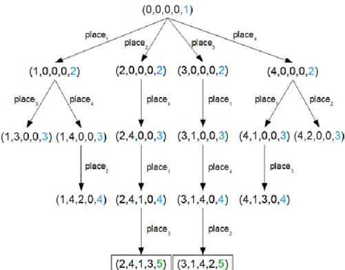
State-space graph. The state-space graph of the aforementioned state-space representation for the case N=4 case can be seen in Figure 4. In this case, the problem has 2 solutions.

Notice that every solution of the problem is N long for sure. It is also important to note that there is no cycle in the state-space graph, that is, by carefully choosing the elements of the state-space representation, we have managed to exclude cycles from the graph, which will be quite advantageous when we are searching solutions.

(21)

Figure 4. The state-space graph of the 4 Queens problem.

(22)

Chapter 4. Problem-solving methods

Problem-solving methods are assembled from the following components:

• Database: stored part of the state-space graph. As the state-space graph may contain circles (and loops), in the database we store the graph in an evened tree form (see below).

• Operations: tools to modify the database. We usually differentiate two kinds of operations:

• operations originated from operators

• technical operations

• Controller: it controls the search in the following steps:

1. initializing the database,

2. selecting the part of the database that should be modified,, 3. selecting and executing an operation,

4. examining the terminating conditions:

• positive terminating: we have found a solution,

• negative terminating: we appoint that there is no solution.

The controller usually executes the steps between (1) and (4) iteratively.

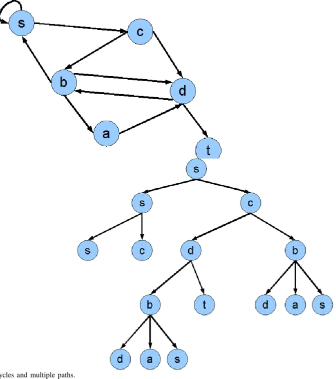
Unfolding the state-space graph into a tree . Let's see the graph on Figure 5. The graph contains cycles, one such trivial cycle is the edge from s to s or the path (s, c, b, s) and the path (c, d, b, s, c). We can eliminate the cycles from the graph by duplicating the appropriate vertices. It can be seen on Figure 6, for example, we eliminated the edge from s to s by inserting s to everywhere as the child of s. The (s, c, b, s) cycle appears on the figure as the rightmost branch. Of course, this method may result in an infinite tree, so I only give a finite part of it on the figure.

(23)

Figure 5. A graph that contains

cycles and multiple paths.

Figure 6. The unfolded tree version.

After unfolding, we need to filter the duplications on the tree branches if we want the solution seeking to terminate after a limited number of steps. That's we will be using different cycle detection techniques (see below) in the controller.

Although, they do not endanger the finiteness of the search, but the multiple paths in the state-space graph do increase the number of vertices stored in the database. On Figure 5, for example, the c, d and the c, b, d paths are multiple, as we can use either of them to get from c to d. The c, d and c, b, a, d paths are also multiple in a less trivial way. On Figure 6, we can clearly see what multiple paths become in the tree we got: the vertices get duplicated, although, not on the same branches (like in the case of cycles), but on different branches. For example, the vertex d appears three times on the figure, which is due to the previously mentioned two multiple paths. Note that the existence of multiple paths not only results in the duplication of one or two vertices, but the duplication of some subtrees: the subtree starting at b and ending at the vertices d, a, s appears twice on the figure.

(24)

Problem-solving methods

As I already mentioned, the loops do not endanger the finiteness of the search. But it is worth to use some kind of cycle detection technique in the controller if it holds out a promise of sparing many vertices, as we reduce the size of the database on a large scale and we spare the drive. Moreover, this last thing entails the reduction of the runtime.

The features of problem-solving methods. In the following chapter we will get to know different problem- solving methods. These will differentiate from each other in the composition of their databases, in their operations and the functioning of their controllers. These differences will result in problem-solving methods with different features and we will examine the following of these features in the case of every such method:

• Completeness: Will the problem-solving method stop after a finite number of steps on every state-space representation, will it's solution be correct or does a solution even exist for the problem? More clearly:

• If there is a solution, what state-space graph do we need for a solution?

• If there is no solution, what state-space graph will the problem-solving method need to recognize this?

We will mostly differentiate the state-space graphs by their finiteness. A graph is considered finite if it does not contain a circle.

• Optimality: If a problem has more than one solution, does the problem-solving method produce the solution with the lowest cost?

The classification of problem-solving methods. The problem-solving methods are classified by the following aspects:

• Is the operation retractable?

1. Non-modifiable problem-solving methods: The effects of the operations cannot be undone. This means that during a search, we may get into a dead end from which we can't go back to a previous state. The advantage of such searchers is the simple and small database.

2. Modifiable problem/solving methods: The effects of the operations can be undone. This means that we can't get into a dead end during the search. The cost of this is the more complex database.

• How does the controller choose from the database?

1. Systematic problem-solving methods: Randomly or by some general guideline (e.g. up to down, left to right). Universal problem-solving methods, but due to their blind, systematic search strategy they are ineffective and result in a huge database.

2. Heuristic problem-solving methods: By using some guessing, which is done on the basis of knowledge about the topic by the controller. The point of heuristics is to reduce the size of the database so the problem-solving method will become effective. On the other hand, the quality of heuristics is based on the actual problem, there is no such thing as „universal heuristics”.

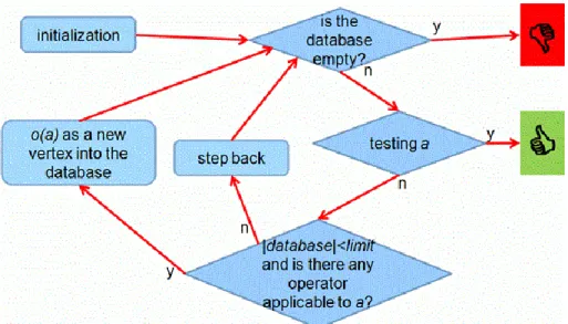
1. Non-modifiable problem-solving methods

The significance of non-modifiable problem-solving methods is smaller, due to their features they can be rarely used, only in the case of certain problems. Their vital advantage is their simplicity. They are only used in problems where the task is not to find a solution (as a sequence of operators), but to decide if there is a solution for the problem and if there is one, than to create a (any kind of) goal state.

The general layout of non-modifiable sproblem-solving methods:

• Database: consists of only one state (the current state).

• Operations: operators that were given in the state-space representation.

• Controller: The controller is trying to execute an operator on the initial state and will overwrite the initial state in the database with the resulting state. It will try to execute an operator on the new state and it will

(25)

again overwrite this state. Executing this cycle continues till the current state happens to be a goal state. In detail:

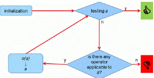
1. Initiating: Place the initial state in the database.

2. Iteration:

a. Testing: If the current state (marked with a) is a goal state then the search stops. A solution exists.

b. Is there an operator that can be executed on a?

• If there isn't, then the search stops. We haven't found a solution.

• If there is, then mark it with o. Let o(a) be the current state.

Figure 7. The flowchart of a non-modifiable problem-solving method.

The features of non-modifiable problem-solving methods:

• Completeness:

• Even if there is a solution, finding it is not guaranteed.

• If there is no solution, it will recognize it in the case of a finite state-space graph.

• Optimality: generating the optimal goal state (the goal state that can be reached by the optimal solution) is not guaranteed.

The certain non-modifiable problem-solving methods differ in the way they choose their operator o for the state a. Wemention two solutions:

1. Trial and Error method: o is chosen randomly.

2. Hill climbing method: We choose the operator that we guess to lead us the closest to any of the goal states.

The magnitude of non-modifiable problem-solving methods is that they can be restarted. If the algorithm reaches a dead end, that is, there is no operator we can use for the current state, then we simply restart the algorithm (RESTART). In the same time, we replenish the task to exclude this dead end (which can be most easily done by replenishing the precondition of the operator leading to the dead end). We set the number of restarts in advance. It's foreseeable that by increasing the number of restarts, the chance for the algorithm to find a solution also increases – provided that there is a solution. If the number of restarts approaches infinity, than the probability of finding a solution approaches 1.

The non-modifiable problem-solving algorithms that use restarts are called restart algorithms.

The non-modifiable problem-solving methods are often pictured with a ball thrown into a terrain with mountains and valleys, where the ball is always rolling down, but bouncing a bit before stopping at the local

(26)

minimum. According to this, our heuristics chooses the operator that brings to a smaller state in some aspect (rolling down), but if there is no such option, than it will randomly select an operator (bouncing) till it is discovered that the ball will roll back to the same place. This will be the local minimum.

In this example, restart means that after finding a local minimum, we throw the ball back again to a random place.

In the restart method, we accept the smallest local minimum we have found as the approached global minimum. This approach will be more accurate if the number of restarts is greater.

The non-modifiable algorithms with restart have great significance in solving the SAT problem. The so- called „random walk” SAT solving algorithms use these methods.

1.1. The Trial and Error method

As it was mentioned above, in the case of the trial and error method, we apply a random operator on the current vertex.

• Optimality: generating the optimal goal state is not guaranteed.

The (only) advantage of the random selection is: the infinite loop is nearly impossible.

Idea: .

• If we get into a dead end, restart.

• In order to exclude getting into that dead end, note that vertex (augment the database).

1.2. The trial and error method with restart

• Database: the current vertex, the noted dead ends, the number of restarts and the number of maximum restarts.

• Controller:

1. Initiating: The initial vertex is the current vertex, the list of noted dead ends is empty, the number of restarts is 0.

2. Iteration: Execute a randomly selected applicable operator on the current vertex. Examine the new state we got whether it is in the list of known dead ends. If yes, then jump back to the beginning of the iteration.

If no, then let the vertex we got be the current vertex.

a. Testing: If the current vertex is a terminal vertex, then the solution can be backtracked from the data written on the screen.

b. If there is no applicable operator for the current vertex, so the current vertex is a dead end:

• If we haven't reached the number of maximum restarts, the we put the found dead end into the database, increase the number of restarts by one, let the initial vertex be the current vertex, and jump to the beginning of the iteration.

• If the number of maximum restarts have been reached, then write that we have found no solution.

The features of the algorithm:

(27)

• The greater the number of maximum restarts is, the better the chances are to find the solution. If the number of restarts approaches infinity, then the chance of finding a solution approaches 1.

• If there is no solution, it will recognize it.

The trial and error algorithm has theoretical significance. The method with restart is called „random walk”. The satisfiability of conjunctive normal forms can be most practically examined with this algorithm.

1.3. The hill climbing method

The hill climbing method is a heuristic problem-solving method. Because the distance between a state and goal state is guessed through a so-called heuristics. The heuristics is nothing else but a function on the set of states (A) which tells what approximately the path cost is between a state and the goal state. So:

Definition 7. The heuristics given for the state-space representation is a function, that h(c)=0

The hill climbing method uses the applicable operator o for the state a where h(o(a)) is minimal.

Let's see how the hill climbing method works in the case of the Towers of Hanoi! First, give a possible heuristics for this problem! For example, let the heuristics be the sum of the distance of the discs from rod R So:

(4.1)

where R-P=2, R-Q=1, and R-R=0 Note that for the goal state (R, R, R), h=(R, R, R)=0 holds.

Initially, the initial state (P, P, P) is in the database. We can apply either the operator move1,Q or move1,R . The first one will result in the state (Q, P, P) with heuristics 5, and the later one will result in (R, P, P) with 4. So (R, P, P) will be the current state. Similarly, we will insert (R, Q, P) into the database in the next step.

Next, we have to choose between two states: we insert either (R, P, P) or (Q, Q, P) into the database. The peculiarity of this situation is that the two states have equal heuristics, and the hill climbing method doesn't say a thing about how to choose between states having the same heuristics. So in this case, we choose randomly between the two states. Note that, if we chose (R, P, P), then we would get back to the previous state, from where we again get to (R, Q, P), where we again step to (R, P, P), and so on till the end of times. If we choose (Q, Q, P) now, then the search can go on a hopefully not infinite branch.

(28)

Going on this way, we meet a similar situation in the state (R, Q, R), as we can step to the states (Q, Q, R) and

(R, P, R) with equal heuristics. We would again run into infinite execution with the first one.

We have to say that we need to be quite lucky with this heuristics for hill climbing method even to stop. Maybe, a more sophisticated heuristics might ensure this, but there is no warranty for the existence of such heuristics.

All in all, we have to see that without storing the past of the search, it's nearly impossible to complete the task and evade the dead ends.

Note that the Towers of Hanoi is a typical problem for which applying a non-modifiable problem-solving method is pointless. The (only one) goal state is known. In this problem, the goal is to create one given solution and for this a non-modifiable method is inconvenient by its nature.

1.4. Hill climbing method with restart

The hill climbing method with restart is the same as the hill climbing method with the addition that we allow a set number of restarts. We restart the hill climbing method if it gets into a dead end. If it reaches the maximum number of restarts and gets into a dead end, then the algorithm stops because it haven't found a solution.

It is important for the algorithm to learn from any dead end, so it can't run into the same dead end twice.

Without this, the heuristics would lead the hill climbing method into the same dead end after a restart, except if the heuristics has a random part. The learning can happen in many ways. The easiest method is to change the state-space representation in a way that we delete the current state from the set of states if we run into a dead end. Another solution is to expand the database with the list of forbidden states.

It is worth to use this method if

1. either it learns, that is, it notes the explored dead ends, 2. or the heuristics is not deterministic.

2. Backtrack Search

One kind of the modifiable problem-solving methods is the backtrack search, which has several variations. The basic idea of backtrack search is to not only store the current vertex in the database, but all the vertices that we used to get to the current vertex. This means that we will store a larger part of the state-space graph in the database: the path from the initial vertex to the current vertex.

The great advantage of backtrack search is that the search can't run into a dead end. If there is no further step forward in the graph from the current vertex, then we step back to the parent vertex of the current one and try to another direction from there. This special step – called the back-step – gave the name of this method.

It is logical that in the database, besides the stored vertex's state, we also need to store the directions we tried to step to. Namely, in every vertex we have to register those operators that we haven't tried to apply for the state stored in the vertex. Whenever we've applied an operator to the state, we delete it from the registration stored in the vertex.

(29)

2.1. Basic Backtrack

• Database: the path from the initial vertex to the current vertex, in the state-space graph.

• Operations:

• Operators: they are given in the state-space representation.

• Back-step: a technical operation which means the deleting of the lowest vertex of the path stored in the database.

• Controller: Initializes the database, executes an operation on the current vertex, tests the goal condition, and decides if it stops the search or re-examines the current vertex. The controller's action in detail:

1. Initialization: Places the initial vertex as the only vertex in the database. Initial vertex = initial state + all the operators are registered.

2. Iteration:

a. If the database is empty, the search stops. We haven't found a solution.

b. We select the vertex that is at the bottom of the path (the vertex that was inserted at latest into the database) stored in the database; we will call this the current vertex. Let us denote the state stored in the current vertex with a !

c. Testing: If a is a goal state then the search stops. The solution we've found is the database itself (as a path).

d. Examines if there is an operator that we haven't tried to apply to a . Namely, is there any more operators registered in the current vertex?

• If there is, denote it with o ! Delete o from the current vertex. Test o 's precondition on a . If it holds then apply o to a and insert the resulted state o(a) at the bottom of the path stored in the database. In the new vertex, besides o(a), register all the operators.

• If there isn't, then the controller steps back.

Figure 8. The flowchart of the basic backtrack method.

The backtrack search we have got has the following features:

• If there is a solution, it will find it in a finite state-space graph.

(30)

Implementation questions.

• What data structure do we use for the database?

Stack.

The operations of the method can be suited as the following stack operations:

• applying an operator: PUSH

• back-step: POP

• In what form do we register the operators in the vertices?

1. We store a list of operators in each vertex.

In this stack, 3 vertices of the 3- mugs-problem can be seen. We have tried to apply the operators pour3,1 and pour3,2 to the initial vertex (at the bottom). We have got the 2^nd vertex by applying pour3,2 , and we only have the operators pour1,2 and pour3,1 left. By applying pour2,1 , we have got the 3^rd (uppermost, current) vertex, to which we haven't tried to apply any operator.

Idea: when inserting a new state, don't store all the operators in the new vertex's list of operators, only those that can be applied to the given state. We can save some storage this way, but it can happen that we needlessly test some operators' precondition on some states (as we may find the solution before their turn).

2. We store the operators outside the vertices in a constant array (or list). In the vertices, we only store the operator indices, namely the position (index) of the operator in the above mentioned array. The advantage of this method is that we store the operators themselves ain one place (there is no redundancy).

(31)

In the case of the 3-mugs-problem, the (constant) array of the operators consists of 6 elements. In the vertices, we store the indices (or references) of the not-yet-used operators.

3. We can further develop the previous solution by that we apply the operators on every state in the order of their position they occur in the array of operators. With this, we win the following: it's completely enough to store one operator index in the vertices (instead of the aforementioned list of operators). This operator index will refer to the operator that we will apply next to the state stored in the vertex. In this way, we know that the operators on the left of the operator index in the array of operators have already been applied to the state, while the ones on the right haven't been applied yet.

We haven't applied any operator to the current vertex, so let its operator index be 1, noting that next time we will try to apply the operator with index 1.

To the 2^nd vertex, we tried to apply the operators in order, where pour2,1 was the last one (the 3^rd operator).

Next time we will try the 4th one.

We have tried to apply all the operators to the initial vertex, so its operator index refers to a non-existent operator.

The precondition of the back-step can be very easily defined: if the operator index stored in the current vertex is greater than the size of the operators' array, then we step back.

Example:

In case of the Towers of Hanoi problem, the basic backtrack search will get into an infinite loop, as sooner or later the search will stuck in one of the cycles of the state-space graph. The number of operator executions depends on the order of the operators in the operators' array.

On Figure 9, we show a few steps of the search. In the upper left part of the figure, the operators' array can be seen. We represent the stack used by the algorithm step by step, and we also show the travelled path in the state- space graph (see Figure 3).

As it can be seen, we will step back and forth between the states (R, P, P) and the (Q, P, P) while filling up the stack. This happens because we have assigned a kind of priority to the operators, and the algorithm is strictly using the operator with the highest priority.

(32)

Figure 9. The basic backtrack in the case of the Towers of Hanoi.

2.2. Backtrack with depth limit

One of the opportunities for improving the basic backtrack method is the expansion of the algorithm's completeness. Namely, we try to expand the number of state-space graphs that the algorithm can handle.

The basic backtrack method only guarantees stopping after a limited amount of steps in case of a finite state- space graph. The cycles in the graph endanger the finite execution, so we have to eliminate them in some way.

We get to know two solutions for this: we will have the backtrack method combined with cycle detection in the next chapter, and a more simple solution in this chapter, that does not eliminate the cycles entirely but allows to walk along them only a limited number of times.

We achieve this with a simple solution: maximizing the size of the database. In a state-space graph it means that we traverse it only within a previously given (finite) depth. In implementation, it means that we specify the

(33)

maximum size of the stack ain advance. If the database gets „full” in this sense during the search, then the algorithm steps back.

So let us specify an integer limit > 0. We expand the back-step precondition in the algorithm: if the size of the database has reached the limit, then we take a back-step.

Figure 10. The flowchart of the backtrack method with depth limit.

The resulting backtrack method's features are the following:

• If there is a solution and the value of the limit is not smaller than the length of the optimal solution, then the algorithm finds a solution in any state-space graph. But if we chose the limit too small, then the algorithm doesn't find any solution even if there is one for the problem. In this sense, backtrack with depth limit does not guarantee a solution.

• If there is no solution, then it will recognize this fact in the case of any state-space graph.

Example . On figure 11, we have set a depth limit, which is 7. The depth limit is indicated by the red line at the top of the stack on the figure. Let us continue the search from the point where we finished it on Figure 11, namely the constantly duplicating of the states (R,P,P) and (Q,P,P). At the 7^th step of the search, the stack's size reaches the depth limit, a back-step happens, which means deleting the vertex on the top of the stack and applying the next applicable operator to the vertex below it. As it is clearly visible, the search gets out of the infinite execution, but it can also be seen that it will take tons of back-steps to head forth the goal vertex.

Note that if we set the depth limit lower than 7, then the algorithm would not find a solution!

(34)

Figure 11. Backtrack with depth limit in the case of the Towers of Hanoi.

2.3. Backtrack with cycle detection

For ensuring that the search is finite, another method is the complete elimination of the cycles in the state-space graphe. It can be achieved by introducing an additional test: a vertex can only be inserted as a new one into the database if it hasn't been the part of it yet. That is, any kind of duplication is to be eliminated in the database.

(35)

Figure 12. The flowchart of the backtrack algorithm with cycle detection.

The resulting problem-solving method has the best features regarding completeness:

• If there is a solution, the algorithmfinds it in any state-space graph.

• If there is no solution, the algorithm realizes this fact in the case of any state-space graph.

• Optimality: finding the optimal solution is not guaranteed.

The price of all these great features is a highly expensive additional test. It's important to only use this cycle detection test in our algorithm if we are sure that there is a cycle in the state-space graph. It is quite an expensive amusement to scan through the database any time a new vertex is getting inserted!

Example . In Figure 13, we can follow a few steps of the backtrack algorithm with cycle detection, starting from the last but one configuration in Figure 9. Among the move attempts from the state (Q,P,P) , there are operators through1,R and through1,P , but the states (R,P,P) and (P,P,P) created by them are already in the stack, so we don't put them in again. This is how we reach the operator through2,R , which creates the state (Q,R,P) , that is not part of the stack yet.

This is the spirit the search is going on, eliminating the duplications in the stack completely. It's worthwhile to note that although the algorithm cleverly eliminates cycles, it reaches the goal vertex in a quite dumb way, so the solution it finds will be far from optimal.

(36)

Figure 13. Backtrack with circle-checking in the case of the Towers of Hanoi.

2.4. The Branch and Bound algorithm

We can try to improve the backtrack algorithm shown in the last chapter for the following reason: to guarantee the finding of an optimal solution! An idea for such an improvement arises quite naturally: the backtrack algorithm should perform minimum selection in the universe of possible solutions.

So, the algorithm will not terminate when it finds a solution, but will make a copy of the database (the vector called solution will be used for this purpose), then steps back and continues the search. It follows that the search will only end if the database gets empty. As we don't want to traverse the whole state-space graph for this, we are going to use a version of the backtrack algorithm with depth limit in which the value of the limit dynamically changes. Whenever finding a solution (and storing it in the vector solution), the limit's new value will be the length of the currently found solution! So, we won't traverse the state-space graph more deeply than the length of the last solution.