On ﬁrst-order methods in stochastic programming

(1)

On first-order methods in stochastic programming

Dissertation submitted for the degree Doctor of the Hungarian Academy of Sciences

Csaba I. F´ abi´ an

John von Neumann University, Kecskem´ et

2019.

(2)

(3)

Foreword

This dissertation covers twenty years of my pursuits in stochastic programming.

They started with a collaboration with András Prékopa. He invited me to im- plement a method of his, and in the course of this collaboration I got acquainted with a discipline I found new and fascinating. (The results of this project were published in the joint paper [61].) During this visit I also got acquainted with an optical fiber manufacturing problem that András was then studying. My PhD dissertation [50] was written about this work, and András was my su- pervisor. On his advice, I started studying bundle methods from a stochastic programming point of view. (Direct results of this line of research are recounted in Chapter 2.) It was due to András’s influence that I gave up a career in IT management for one in the academic sphere, a decision I’ve never regretted.

As I had an informatics background, I went into computational stochastic programming. My results extensively rely on the achievements of András and of members of his school: István Deák, János Mayer and Tamás Szántai.

In the years 2007-2010 I collaborated with Gautam Mitra and his team at Brunel University. As a visiting researcher, I spent a month in each of these years at Brunel. Also went to conferences and workshops with that team. I owe many academic acquaintances to Gautam. It was due to him that I got involved in coordination activities of the Stochastic Programming Society. Since Gautam’s retirement, I have been collaborating with Achim Koberstein and his colleagues from Paderborn University and the European University Viadrina.

I owe much to the academic leadership of the John von Neumann Univer- sity, former Kecskemét College, and to my senior colleagues there. They have always strived to provide the conditions of research. Helping young colleagues at Kecskemét is a pleasant obligation for me. One of our projects involves probabilistic problems. Providentially, we can collaborate with Tamás Szántai.

I’m grateful to colleagues and friends in the Hungarian operations research community for encouragement and advice. Especially, I’m obliged to Aur´el Gal´antai who has from time to time read the current versions of my materials and recommended improvements.

(4)

(5)

Introduction

The importance of making sound decisions in the presence of uncertainty is clear in everyday life. Wodehouse in [182], Chapter 6, advocates ‘a wholesome pessimism, which, though it takes the fine edge off whatever triumphs may come to us, has the admirable effect of preventing Fate from working off on us any of those gold bricks, coins with strings attached, and unhatched chickens, at which Ardent Youth snatches with such enthusiasm, to its subsequent disappointment.’

Advancing age, Wodehouse points out, brings forth prudence. The discipline of stochastic programming promises a faster track.

According to a widely accepted definition, stochastic programming handles mathematical programming problems where some of the parameters are random variables. The Stochastic Programming Society (which exists as a Technical Section of the Mathematical Optimization Society) defines itself as ’a world- wide group of researchers who are developing models, methods, and theory for decisions under uncertainty’. Our approach involves the characterization and modeling of the distribution of the random parameters, and the measuring of risks. The ensuing options may make model building a challenge.

We get a more complete picture of the field by a survey of the achievements that are generally accepted as landmarks. The Stochastic Programming Soci- ety honors twelve outstanding researchers with the title ’Pioneer of Stochastic Programming’. I excerpt from the laudations with a focus on theoretic results and applications.

George Dantzig introduced linear programming under uncertainty, present- ing the simple recourse model, the two-stage stochastic program and the multi-stage stochastic program. He developed, with A. Madansky, the first decomposition method to solve two-stage stochastic linear programs.

He very early foresaw the importance of sampling methods, and later (with P.W. Glynn and G. Infanger) contributed to the development of them. Dantzig’s discoveries were continually motivated by applications.

His seminal work has laid the foundation for much of the field of systems engineering and is widely used in network design and component design in

(8)

computer, mechanical, electrical engineering. He also developed applications for the oil industry (with P. Wolfe), and in aircraft allocation (with A.R. Ferguson).

Michael Dempster studied the solvability of two-stage stochastic programs and provided a bridge between stochastic programming and related statistical decision problems. He also introduced the use of interval arithmetic to SP. In collaboration with J. Birge, G. Gassman, E. Gunn, A. King, and S.

Wallace, he participated in the creation of the SMPS standard, the most widely-used data format for SP instances. For decades, he has worked on SP applications in scheduling, finance, and other areas.

Jitka Dupaˇcov´a proposed a new decision model for the handling of incomplete distributional information. Her minimax approach was one of the fore- bears of the recent branch of distributionally robust optimization. She also developed the contamination technique that facilitates stability analysis. She made important contributions to asymptotics (including work with R. Wets), and scenario selection/reduction (including work with W.

R¨omisch, G. Consigli, and S. Wallace). She extensively contributed to applications; in economics and finance (including work with M. Bertocchi), water management (including work with Z. Kos, A. Gaivoronski and T.

Sz´antai), and industrial processes (including work with P. Popela).

Yuri Ermoliev with his students has been the major proponent of the stochastic quasigradient method. This approach enables the approximate solution of difficult SP problems. He suggested (with N. Shor) a stochastic analogue of the subgradient process for solving two-stage stochastic programing problems. He worked (with V. Norkin) on measuring, profiling and man- aging catastrophic risks. He has also worked on other fields of application:

pollution control problems, energy and agriculture modeling.

Peter Kall was one of the principal guiding forces in the development of suc- cessive approximation methods. He developed bounding approaches with K. Frauendorfer. He developed and promoted, with J. Mayer, the stochastic programming solver system SLP-IOR that has been provided free for educational purposes.

Willem K. Klein Haneveld’s early contributions consist of results on marginal problems, moment problems, and dynamic programming. He introduced integrated chance constraints. He was among the first to study stochastic programs with integer variables, both in theory and applications. He worked on SP applications for pension funds and the gas industry.

Kurt Marti has been one of the major proponents of SP approaches to engineering problems, including those arising in structural design and robotics.

He also dealt with approximation and stability issues. He developed new algorithms in semi-stochastic approximation and stochastic quasigradient methods.

(9)

3 András Prékopa introduced probabilistic constraints involving dependent random variables. He developed the theory of logconcave measures, a mo- mentous step in the treatment of probabilistic constraints. Together with I. Deák, J. Mayer and T. Szántai, he developed efficient numerical methods for the solution of probabilistic programming problems. He and his co-workers applied his methodology to water systems and power networks in Hungary, and developed a new inventory model, now known as the Hungarian inventory control model. He also worked on the bounding and approximation of expectations and probabilities in higher dimensional spaces. Applications of this theory include communication and transporta- tion network reliability, the characterization of the distribution function of the length of a critical path in PERT, approximate solution of probabilistic constrained stochastic programming problems, and the calculation of multivariate integrals.

Stephen M. Robinson contributed to the study of error bounds and the continu- ity of solution sets under data perturbations. These results led to his joint work with R. Wets on the stability of two-stage stochastic programs. He has also worked on sample path optimization, and applied these methods to decision models arising in manufacturing and military applications.

R. Tyrell Rockafellar’s fundamental results in convex analysis have been extensively applied in SP. With R. Wets, he studied Lagrange multipliers for nonanticipativity constraints. This prepared the way for their development of the progressive hedging algorithm, in which a Lagrangian relaxation of the nonanticipativity constraints allows the use of determin- istic solvers. With S. Uryasev and W.T. Ziemba, he has contributed to the foundation of risk management in finance.

Roger J.B. Wets presented work on model classes and properties of these classes (particularly with D. Walkup), and basic algorithmic approaches for solving these models – particularly the L-shaped method (with R. Van Slyke).

His early work on underlying structures (with C. Witzgall) later led to many algorithmic developments and preprocessing procedures. He recog- nized that nonanticipativity can be expressed as constraints, later leading to the progressive hedging algorithm (with R.T. Rockafellar). He has also examined statistical properties of stochastic optimization problems, generalizing the law of large numbers, justifying the use of sampling in solving stochastic programs. He was instrumental in the development of epi/hypo-convergence, approximations and also sampling. Throughout his career, he has been involved in applications of stochastic programming.

His first large, and well-known, application is that of lake eutrophication management in Hungary (with L. Somly´ody).

William T. Ziemba is interested in the applications of SP, in particular to portfolio selection in finance. Since 1983 he has been a futures and equity trader and hedge fund and investment manager. He was also instrumental

(10)

in the most successful commercial application of SP to a Japanese insur- ance company, Yasuda Kasai. He is also noted for his applications of SP to race track betting, energy modelling, sports and lottery investments.

The achievements of András Prékopa and his co-workers have a special importance to us. With Tamás Szántai, they developed a stochastic programming model for the optimal regulation of storage levels, and applied it to the water level regulation of lake Balaton. (In connection with this project, they developed a new multidimensional gamma distribution.) With Tamás Szántai, Tamás Rapcsák and István Zsuffa, they developed models for the optimal design and operation of water storage and flood control reservoir systems. He led a project for MVM (Hungarian Electrical Works) for the optimal daily scheduling of power generation. His co-workers were János Mayer, Beáta Strazicky, István Deák, János Hoffer, Ágoston Németh and Béla Potecz. In another project with Sándor Ganczer, István Deák and Károly Patyi, they applied his STABIL model to the electrical energy sector of the Hungarian economy. They were able to dra- matically increase the reliability level of the Hungarian power network without cost increase. With Margit Ziermann, he developed the Hungarian inventory control model whose re-ordering rules allowed a substantial decrease in inventory levels.

The stochastic programming school established by András Prékopa is recog- nized and appreciated by the SP community world-wide. Each of their projects included the development of novel theoretical results, new models and algorithms as well as the implementation of the appropriate solvers. — In Section 7.2, I’ll give an overview of the methods and solvers they developed for the solution of probabilistic constrained problems. These solution methods need an oracle that computes or estimates distribution function values and gradi- ents. An abundant stream of research in this direction has been initiated by the work of Prékopa and his school. In Section 7.3, I’ll give an overview of these estimation methods.

I mention a further project, the development of a pavement management system for the allocation of financial resources to maintenance and reconstruc- tion works on Hungary’s road network. The pavement management system was based on stochastic models, and was developed by András Bakó, Emil Klafszky, Tamás Szántai and László Gáspár. Though I had not yet been acquainted with stochastic programming at the time, I was involved indirectly. They applied my linear programming solver for the solution of the LP equivalents of their stochastic programming problems.

*

I perceive the following recent developments and trends in the stochastic programming field.

Multi-stage models and solution methods have become a heavy-duty tool, especially in energy planning. Effective solution methods have been known for decades, but theoretical justification of multi-stage models was missing. Just a

(11)

5 decade ago, many of us had doubts whether accuracy in the modelling of the random process is compatible with solvability. Recent results in scenario-tree approximation show they are. Paradoxical features of risk measurement in mul- tistage models have been clarified, and safe frameworks have been established.

A new branch has been developing under the name of distributionally robust optimization. The motivation is that the distribution of the random parameters is rarely known in the explicit form required by classic models. We may not even have enough data for a sampling approach, but may know that the distribution belongs to a certain class. The idea is to focus on the worst distribution belonging to that class. (This is analogous to plain robust optimization but avoids over-simplification resulting in over-conservative decisions.) This new modelling approach is inherently related to risk constraints, through duality.

Equilibrium models have appeared in stochastic programming. This is probably due to the de-regulation of the energy markets in Western economies. Given an environment of regulations, resources and random demands, energy produc- ers are expected to compete, and production decisions are modelled on the principles of game theory. Most interesting is the problem of the regulator, who exercises its (limited) influence to steer investment decisions towards a desirable course.

*

This dissertation focusses on computational aspects. Functions involving expectations, probabilities and risk measures typically occur in stochastic programming problems. This means large amounts of data to be organized, and inaccuracy in function evaluations. Interestingly, similar solution approaches proved effective for very diverse problems; enhanced cutting-plane methods in primal and dual forms. I discuss cutting-plane methods in Chapter 2, and their application to the handling of risk measures in Chapter 3.

Decomposition has originally been proposed to overcome the bottleneck of restricted memory. Memory is no longer a scarce resource (entire databases are handled in-memory on today’s computers), but decomposition is still relevant, as I’m going to demonstrate in Chapters 4, 5 and 6.

Probabilities are one of the oldest and most intuitive means of controlling risk (you need not explain the concept of ’chance’ to a decision maker.) Probabilistic programming is still in the focus of research. I present an overview of current developments in Chapter 7.

The importance of sampling-based methods have significantly increased in recent years, and further hard problems are being attacked by such methods. In Chapter 8, I recount a randomized method bearing a resemblance to stochastic gradient methods. In Chapter 9, I apply this method in an approximation scheme for handling a difficult constraint. In Chapter 10, I adapt the randomized method of Chapter 8 to probability maximization.

(12)

(13)

Chapter 2

Cutting-plane methods and enhancements

In this chapter we deal with special solution methods for the unconstrained problem

minϕ(x) such that x∈X, (2.1)

and the constrained problem

minϕ(x) such that x∈X, ψ(x)≤0, (2.2) where X ⊂ IRⁿ is a convex bounded polyhedron with diameter D, and ϕ, ψ are IRⁿ→IR convex functions, both satisfying the Lipschitz condition with the constant Λ. We assume that ψtakes positive values as well as 0.

In our contextX is explicitly known. The functions, on the other hand, are not known explicitly, but we have an oracle that returns function values and a subgradients at any given point.

A cutting-plane method is an iterative procedure based on polyhedral models. Suppose we have visited iterates x1, . . . ,xi. Having called the oracle at these iterates, we obtained linear supporting functions lj(x) (1≤j ≤i), i.e.,

l_j(x)≤ϕ(x) (x∈IRⁿ) and l_j(x_j) =ϕ(x_j). (2.3) The current polyhedral model function is the upper cover of these supporting functions,

ϕi(x) = max

1≤j≤i lj(x) (x∈IRⁿ). (2.4) A cutting-plane model ofψ is also built in a similar manner:

ψi(x) = max

1≤j≤il⁰_j(xj) (x∈IRⁿ), (2.5) where l⁰_j is a supporting linear function toψ(x) atx_j (j = 1, . . . , i).

Using these objects, a model problem is constructed:

minϕi(x) such that x∈X, ψi(x)≤0, (2.6) and the next iterate will be a minimizer of the model problem.

(14)

2.1 Historical perspectives

Cutting-plane methods for convex problems were proposed by Kelley [87], and Cheney and Goldstein [22] in 1959-1960. These methods are considered fairly efficient for quite general problem classes. However, according to my knowledge, efficiency estimates only exist for the continuously differentiable, strictly convex case. An overview can be found in Dempster and Merkovsky [36], where a geometrically convergent version is also presented.

Though fairly efficient in general, cutting-plane methods are notorious for zigzagging, a consequence of linear approximation. Moreover, starting up is often cumbersome, and cuts tend to become degenerate by the end of the process.

To dampen zigzagging, a natural idea is centralization. It means maintaining a localization set, i.e., a bounded polyhedron that contains the minimizers of the convex problem. A ’central’ point in the polyhedron is then selected as the next iterate.

I sketch the procedure as applied to the unconstrained problem (2.1), and in a form that best suits to forthcoming discussions. After theith iteration, let the localization polyhedron be

P_i= (x, φ)

x∈X, ϕ_i(x)≤φ≤φ_i ,

whereφ_i denotes the best function value known at this stage of the procedure.

The next iterate will then be the x-component of a center of Pi. Different centers have been proposed and tried. The earliest one was the center of gravity by Levin [100]. Applications of this variant have been hindered by the difficulty of computing the center of gravity.

The center of the largest inscribed ball, due to Elzinga and Moore [47], resulted in a successful variant. A more general version, based on the center of the largest-volume inscribed ellipsoid was proposed by Vaidya [171].

The center most used nowadays is probably the analytic center that was introduced by Sonnevend in [158], and has roots in control theory. A cutting- plane method based on the analytic center was proposed by Sonnevend [159].

The method was further developed by Goffin, Haurie, and Vial [71].

2.2 Regularized cutting-plane methods

The following discussion is focused on the unconstrained problem, and I’ll treat the constrained problem as an extension.

Regularized cutting-plane approaches have been developed in the nineteen seventies. I sketch the bundle method of Lemar´echal [98], noting that the method is closely related to the proximal point method of Rockafellar [141].

The idea is to maintain a stability center, that is, to distinguish one of the iterates generated that far. The stability center is updated every time a significantly better iterate was found. Roaming away from the current stability center is penalized. Formally, let x^◦_i denote the stability center after the ith

(15)

2.2. REGULARIZED CUTTING-PLANE METHODS 9 iteration. The next iterate x_i+1 will be an optimal solution of the penalized model problem

xmin∈X

n

ϕi(x) +ρi

2kx−x^◦_ik²o

, (2.7)

where ρi > 0 is a penalty parameter. xi+1 is often called test point in this context, and the solution is approximated by the sequence of stability centers.

As for the new stability center, let

x^◦_i+1=







xi+1 if the new iterate is significantly better thanx^◦_i, x^◦_i otherwise.

(2.8)

In the former case,x^◦_i →x^◦_i+1is called a null step; in the latter, a descent step.

Two issues need further specification: adjustment of the penalty parameter, and interpretation of the term ’significantly better’ in the decision about the stability center. Schramm and Zowe [153] discuss these issues and present convergence statements applying former results of Kiwiel [90].

The level method of Lemar´echal, Nemirovskii and Nesterov [99] uses level sets of the model function to regularize the cutting-plane method. Having performed theith iteration, let

φ_i= min

1≤j≤i ϕ(xj) and φ_i= min

x∈X ϕi(x). (2.9) These are respective upper and lower bounds for the minimum of the convex problem (2.1). Let ∆_i =φ_i−φ

i denote the gap between these bounds. (The sequence of the upper bounds being monotone decreasing, and that of the lower bounds monotone increasing, the gap is tightening at each step.) Let us consider the level set

X_i =n

x∈X|ϕ_i(x)≤φ

i+λ∆_io

(2.10) where 0< λ <1 is a level parameter. The next iterate is computed by projecting xi onto the level setXi. That is,

xi+1= arg min x∈Xi

kx−xik², (2.11)

where k.k means Euclidean norm. Setting λ= 0 gives the pure cutting-plane method. With non-extremal setting, the level sets stabilize the procedure. (The level parameter needs no adjusting in the course of the procedure. That is in contrast with general bundle methods.)

Definition 1 Critical iterations. Let us consider a maximal sequence of iterations x1→ · · · →xssuch that ∆1≥ · · · ≥∆s≥(1−λ)∆1 holds. Maximality of this sequence means that (1−λ)∆1 >∆s+1. Then the iteration xs→xs+1

is labelled critical. This construction is repeated starting from the index s+ 1.

Thus the iterations are grouped into sequences, and the sequences are separated with critical iterations.

(16)

Remark 2 Let ∆⁽ⁱ⁾ denote the gap after the ith critical iteration. We have (1−λ)∆⁽ⁱ⁾ > ∆⁽ⁱ⁺¹⁾ by definition, and hence (1−λ)ⁱ∆⁽¹⁾ > ∆⁽ⁱ⁺¹⁾. The number of critical iterations needed to decrease the gap below is thus on the order of log(1/).

Given a sequencext→ · · · →xsof non-critical iterations, it turns out that the iterates are attracted towards a point that we can call stability center. (Namely, any point from the non-empty intersectionXt∩ · · · ∩Xsis a suitable stability center. Hence we can look on the level method as a bundle-type method.) Using these ideas, Lemar´echal, Nemirovskii and Nesterov proved the following efficiency estimate. Let > 0 be a given stopping tolerance. To obtain a gap smaller than, it suffices to perform

c(λ) ΛD

²

(2.12) iterations, wherec(λ) is a constant that depends only onλ. Even more important is the following experimental fact, observed by Nemirovski in [112], Section 8.2.2. When solving a problem of dimensionnwith accuracy, the level method performs no more than

nln V

(2.13) iterations, whereV = maxXϕ−minXϕ is the variation of the objective over X, that is obviously over-estimated by ΛD. Nemirovski stresses that this is an experimental fact, not a theorem; but he testifies that it is supported by hundreds of tests.

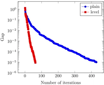
I illustrate practical efficiency of the level method with two figures taken from our computational study [190] where we adapted the level method to the solution of master problems in a decomposition scheme. Figures 2.1 and 2.2 show the progress of the plain cutting-plane method vs the level method in terms of the gap. The gap is measured on a logarithmic scale.

These figures well represent our findings. Cuts in the plain method tend to become shallow, as in Figure 2.1, while the level method shows a steady progress. Moreover, initial iterations of the plain method are often ineffective, as shown in Figure 2.2. Starting up causes no problem for the level method.

Remark 3 All the above discussion about the level method and the corresponding results remain valid if the lower boundsφ_i(i= 1,2, . . .)in (2.9) are not set to be respective minima of the related model functions, but set more generally, observing the following rules:

the sequence φ

i is monotone increasing, and xmin∈Xϕ_i(x) ≤ φ

i ≤ φ_i holds for everyi.

(17)

2.2. REGULARIZED CUTTING-PLANE METHODS 11

0 100 200 300 400

10⁻⁶ 10⁻⁵ 10⁻⁴ 10⁻³ 10⁻² 10⁻¹ 10⁰

Number of iterations

Gap

plain level

Figure 2.1: Decrease of the gap: plain cutting-plane method vs level method

20 40 60 80 100 120

10⁻⁶ 10⁻⁵ 10⁻⁴ 10⁻³ 10⁻² 10⁻¹ 10⁰ 10¹

Number of iterations

Gap

plain level

Figure 2.2: Decrease of the gap: plain cutting-plane method vs level method

(18)

Lemar´echal, Nemirovskii and Nesterov extended the level method to the solution of the constrained problem (2.2). Their constrained level method is a primal-dual method, where the dual variable α∈IR is kept unchanged as long as possible. The procedure consists of runs of an unconstrained method applied to the composite objectiveαϕ(x) + (1−α)ψ(x). – To be precise, we speak of runs of a special unconstrained method that satisfies the criteria of Remark 3.

Let Φ denote the optimal objective value of problem (2.2). If Φ is known in advance, then the quality of an approximate solutionx∈X can be measured by max{ϕ(x)−Φ, ψ(x)}.

Let moreover Φ_i denote the optimal objective value of the model problem (2.6). This is a lower approximation for Φ.

The best point after iteration iis constructed in the form of a convex combination of the former iterates:

x^?_i =

i

X

j=1

%jxj, (2.14)

where the weights are determined through the solution of the following problem min max

( i

P

j=1

%jϕ(xj)−Φ_i,

i

P

j=1

%jψ(xj) )

such that %j ≥0 (j= 1, . . . , i),

i

P

j=1

%j= 1.

(2.15)

The linear programming dual of (2.15) is written as max_α∈[0,1]hi(α) with hi(α) = min

1≤j≤i

α(ϕ(xj)−Φ_i) + (1−α)ψ(xj) . (2.16) The next dual iterate αi is set according to the following construction. Let Ii ⊆[0,1] denote the interval over whichhi(α) takes non-negative values. Let moreover the subinterval Îi⊂Ii be obtained by shrinkingIi: the center of Îi is the same as the center ofIi, and for the lengths,|Iî| = (1−µ)|Ii| holds with some preset parameter 0< µ <1. The rule is then to set

αi=







αi−1 if i >1 and αi−1∈Iˆi, center ofI_i otherwise.

(2.17) The next primal iteratexi+1 is selected by applying a level method iteration to the composite objective functionαiϕ(x) + (1−αi)ψ(x), with the cutting-plane modelαiϕi(x) + (1−αi)ψi(x). The best function value taken among the known iterates isφ_i=αiΦ_i+hi(αi). A lower function level is selected specially as

φi=α_iΦ_i. (2.18)

Using these objects and ideas, Lemar´echal, Nemirovskii and Nesterov proved the following efficiency estimate. Let >0 be a given stopping tolerance. To

(19)

2.3. WORKING WITH INEXACT DATA 13 obtain an -optimal-feasible solution, it suffices to perform

c(µ, λ) 2ΛD

2

ln 2ΛD

(2.19) iterations, wherec(µ, λ) is a constant that depends only on the parameters. The idea of the proof is to divide the iterations into subsequences in whose course the dual iterate does not change. The proof is based on the following propositions.

Proposition 4 Assume that >max_α∈[0,1]hi(α)holds.

Thenx^?_i is an-feasible-optimal solution for the constrained problem (2.2), i.e., x^?_i ∈X, ψ(x^?_i)≤andϕ(x^?_i)≤Φ +.

Proposition 5 hi(αi) ≥ ^µ₂max_α∈[0,1]hi(α) always holds with the dual iterate selected according to (2.17).

Proposition 6 Consider a sequence of iterations in the course of which the dual iterate does not change; namely, let t < s be such thatαt=· · ·=αs.

If s−t > c(λ) ^ΛD_ε ²

holds with some ε >0, then hs(αs) ≤ ε follows. – Here c(λ)is the constant of the efficiency estimate (2.12).

Proposition 7 Let 1< t < sbe such thatα_t−16=αt=· · ·=α_s−16=αs. Then|It| ≥(2−µ)|Is| holds due to the selection rule of the dual iterate.

The key is Proposition 6 that is a consequence of the efficiency estimate (2.12) of the level method. The specially selected lower levels (2.18) satisfy the rules of Remark 3.

2.3 Working with inexact data

Exact supporting functions of the form (2.3) are often impossible to construct, or may require an excessive computational effort. A natural idea is to construct approximate supporting functions. Given the current iterate ˆxand the accuracy tolerance ˆδ >0, let the oracle return a linear function satisfying

`(x)≤ϕ(x) (x∈IRⁿ) and `(ˆx)≥ϕ(ˆx)−ˆδ. (2.20) The simplest idea is to construct a sequenceδi&0 before optimization starts.

In the course of the ith oracle call, the accuracy tolerance ˆδ=δi will then be prescribed. Zakeri, Philpott and Ryan [187] applied this approach to the pure cutting-plane method, others to bundle methods.

Kiwiel [89] developed an inexact bundle method, where ’the accuracy tolerance is automatically reduced as the method proceeds. The reduction is, on the one hand, slow enough to save work by allowing inexact evaluations far from a solution, and, on the other hand, sufficiently fast to ensure that the method generates a minimizing sequence of points.’ At each iteration, Kiwiel estimates the quantity by which the new test point can improve on the current stability

(20)

center. He regulates accuracy by halving the oracle tolerance every time it is found too large as compared to this estimate of potential improvement.

In [51], I developed an approximate version of the level method. The idea was to always set the accuracy tolerance in proportion to the current gap. — The method was called ’inexact’ in the paper. In view of future developments, though, I’m going to call it ’approximate’ in this dissertation. — I extended the convergence proof of Lemar´echal, Nemirovskii and Nesterov [99] to the approximate level method. Subsequent computational studies ([62], [184]) indicate that my approximate level method inherits the experimental efficiency (2.13).

I also worked out an approximate version of the constrained level method, and extended the efficiency estimate (2.19) to the approximate version.

Kiwiel [91] developed a partially inexact version of the bundle method. To- gether with a new test pointxi+1, a descent targetφi+1∈IR is always computed, based on the predicted objective decrease that occurs when moving fromx^◦_i to xi+1. A descent step is taken if ϕ(xi+1) ≤ φi+1, a null step otherwise. The oracle works as follows. Passed the current test point ˆxand descent target ˆφ, it returns a linear function`(x)≤ϕ(x) (x∈IRⁿ) such that

either `(ˆx)>φ,ˆ certifying that the descent target cannot be attained, or `(ˆx)≤φ,ˆ in which case`(ˆx) =ϕ(ˆx) should hold.

(2.21) No effort is devoted to approximating the function at the new test point, if no significant improvement can be expected.

De Oliveira and Sagastiz´abal [27] developed a general approach for the handling of inaccuracy in bundle and level methods. Their analysis ’considers novel cases and covers two particular on-demand accuracy oracles that are already known: the asymptotically exact oracles from [51, 62, 187]; and the partially inexact oracle in [91].’ — In the taxonomy of de Oliveira and Sagastiz´abal, methods that drive the accuracy tolerance to 0 are called ’asymptotically exact’. I’m going to call them ’approximate’ in this dissertation, in accord with the terminology introduced above.

[27] also contains a thorough computational study. The authors solved two- stage stochastic programming problems from the collection of De´ak, described in [33]. A decomposition framework was implemented and the master problems were solved with cutting-plane, bundle and level methods, applying different approaches for the handling of inexact data. Regularized methods performed better than pure cutting-plane methods. Among regularized methods, level methods performed best. Inexact function evaluations proved generally effective. The best means of handling inexact data proved to be a combination of my approximate level method and of Kiwiel’s partially inexact approach. ([27]

won Charles Broyden Prize, awarded annually to the best paper published in the Optimization Methods and Software journal.)

(21)

2.4. RECENT CONTRIBUTION 15

2.4 Recent contribution

In [64] and [184] I worked out a special version of the on-demand accuracy approach of de Oliveira and Sagastiz´abal [27]. — According to the taxonomy of [27], my method falls into the ’partly asymptotically exact’ category, and this term was used also in our papers [64] and [184]. In this dissertation, I’m going to call the method ’partially inexact’ to keep the terminology simple. (The latter term is in accord with Kiwiel’s terminology of [91].)

My specific version is interesting for two reasons. First, it enables the extension of the on-demand accuracy approach to constrained problems. Second, the method admits a special formulation of the descent target (specified in Proposition 11, below). This formulation indicates that the method combines the advantages of the disaggregate and the aggregate models when applied to two-stage stochastic programming problems. (This will be discussed in Chapter 4.)

In the following description of the partially inexact level method, the iterations where the descent target has been attained are called substantial.

Ji ⊂ {1, . . . , i} denotes the set of the indices belonging to substantial iterates up to theith iteration. If thejth iteration is substantial then the accuracy toleranceδj is observed in the corresponding approximate supporting function.

Formally, lj(xj) +δj ≥ϕ(xj) holds for j ∈ Ji. The best upper estimate for function values up to iterationiis

φ_i= min

j∈Ji

{l_j(x_j) +δ_j }. (2.22) The accuracy tolerance is always set to be proportional to the current gap, i.e., we have δi+1=γ∆i with an accuracy regulating parameterγ(0< γ1).

Algorithm 8 A partially inexact level method.

8.0 Parameter setting.

Set the stopping tolerance >0.

Set the level parameterλ(0< λ <1).

Set the accuracy regulating parameterγ such that 0< γ <(1−λ)². 8.1 Bundle initialization.

Leti= 1 (iteration counter).

Find a starting pointx1∈X.

Letl₁(x) be a linear support function to ϕ(x) atx₁. Letδ1= 0 (meaning thatl1is an exact support function).

LetJ₁={1} (set of substantial indices).

8.2 Model construction and near-optimality check.

Letϕi(x) = max

1≤j≤ilj(x) be the current model function.

Computeφ_i= min

x∈X ϕi(x), and letφ_i= min

j∈Ji

{lj(xj) +δj}.

(22)

Let ∆_i=φ_i−φ

i. If ∆_i< then near-optimal solution found, stop.

8.3 Finding a new iterate.

LetX_i=n

x∈X|ϕ_i(x)≤φ

i+λ∆_io . Letxi+1= arg min

x∈Xi

kx−xik². 8.4 Bundle update.

Letδi+1=γ∆i.

Call the oracle with the following inputs:

- the current iteratexi+1,

- the accuracy toleranceδi+1, and - the descent targetφ_i−δi+1.

Letli+1(x) be the linear function returned by the oracle.

If the descent target was reached then let Ji+1=Ji∪ {i+ 1}, otherwise letJi+1=Ji.

Incrementi, and repeat from step8.2.

Specification 9 Oracle for Algorithm 8.

The input parameters are xˆ: the current iterate,

δˆ: the accuracy tolerance, and φˆ: the descent target.

The oracle returns a linear function `(x) such that

`(x)≤ϕ(x) (x∈IRⁿ), k∇`k ≤Λ, and

either `(ˆx)>φ,ˆ certifying that the descent target cannot be attained, or `(ˆx)≤φ,ˆ in which case `(ˆx)≥ϕ(ˆx)−δˆ should also hold.

Theorem 10 To obtain∆i< , it suffices to perform c(λ, γ) ^ΛD ²

iterations, wherec(λ, γ) is a constant that depends only onλandγ.

Proof. This theorem is a special case of Theorem 3.9 in de Oliveira and Sagas- tizábal [27]. – The key idea of the proof is that given a sequencex_t→ · · · →x_s of non-critical iterations according to Definition 1, an upper bound can be given on the length of this sequence, as a function of the last gap ∆s. A simpler proof can be composed by extending the convergence proof of the approximate level method in Fábián [51]. Theorem 7 in [51] actually applies word for word, only (2.22) needs to be substituted for the upper bound. I abstain from including this proof.

The computational study of [184] indicates that the partially inexact level method inherits the experimental efficiency (2.13).

(23)

2.4. RECENT CONTRIBUTION 17 The partially inexact level method admits a special formulation of the descent target. Let

κ= γ

1−λ (2.23)

with the parameters λ, γ set in step 8.0 of Algorithm 8. Of course we have 0< κ <1.

Proposition 11 The efficiency estimate of Theorem 10 remains valid with the descent targetκϕi(xi+1) + (1−κ)φ_i set in step 8.4 of the partially inexact level method.

Proof. Let us first consider the case i >1 and the iteration xi−1 →xi was non-critical according to Definition 1. We are going to show that the descent target remains unchanged in this case, i.e.,

κϕ_i(x_i+1) + (1−κ)φ_i=φ_i−δ_i+1. (2.24) Due to the non-criticality assumption we have (1−λ)∆_i−1≤∆_i. Hence by the definition of δi and the parameter setting γ <(1−λ)² we get

δi=γ∆_i−1≤ γ

1−λ∆i <(1−λ)∆i. (2.25) Let us observe that

ϕi(xi) +δi≥φ_i (2.26)

holds, irrespective of x_i being substantial or not. (In casei ∈ Ji, this follows from the definition ofφ_i; otherwise, a consequence ofφ_i=φ_i−1.)

From (2.26) and (2.25) follows

ϕ_i(x_i)≥φ_i−δ_i> φ_i−(1−λ)∆_i=φ

i+λ∆_i. (2.27) (The equality is a consequence of ∆i=φ_i−φ_i.)

The new iteratexi+1found in step8.3 belongs to the level setXi, hence we have

ϕ_i(x_i+1)≤φ

i+λ∆_i. (2.28)

The functionϕi(x) is continuous, hence due to (2.27) and (2.28) there existsxb∈ [xi,xi+1] such thatϕi(bx) =φ_i+λ∆i. We are going to show that equality holds in (2.28). The assumptionϕi(xi+1)< φ_i+λ∆ileads to a contradiction, because in this case bx ∈ [xi,xi+1) should hold, implying kxi−bxk² < kxi−xi+1k². Obviously bx∈Xi, which contradicts the definition ofxi+1.

Hence we have equality in (2.28). From this and the selection ofκwe obtain κϕi(xi+1) + (1−κ)φ_i = κ

φi+λ∆i

+ (1−κ)φ_i = φ_i−κ(1−λ)∆i, which proves (2.24) due to the setting κ= _1−λ^γ .

Let us now consider the case when the iterationx_i−1→x_i was critical. The upper bound mentioned in the proof of Theorem 10 applies to the sequence of

(24)

non-critical iterations just precedingx_i−1 →x_i. Hence the same estimate applies to the total number of non-critical iterations. (The linear functionl_i+1(x) generated by the modified descent target may prove useless, resulting in an ex- traneous iteration. However, the number of critical iterations is small – on the

order of log(1/) as noted in Remark 2.)

An analogue of Remark 3 holds for the partially inexact level method:

Remark 12 All the above discussion about the partially inexact level method and the corresponding results remain valid if the lower boundsφ

i (i= 1,2, . . .) are not set to be respective minima of the related model functions, but set more generally, observing the following rules: the sequenceφ

i is monotone increasing

; φ

i ≤φ_i holds ; and φ

i is not below the minimum of the corresponding model function overX.

In [64], I extended the on-demand accuracy approach to constrained problems. Letl_j(x) andl⁰_j(x) denote the approximate support functions constructed toϕ(x) andψ(x), respectively, in iterationj. Like in the unconstrained case, we distinguish between substantial and non-substantial iterates. LetJi⊂ {1, . . . , i}

denote the set of the indices belonging to substantial iterates up to theith iteration. Ifj ∈ Jithen we havelj(xj) +δj≥ϕ(xj) andl⁰_j(xj) +δj ≥ψ(xj), with a toleranceδj determined in the course of the procedure.

The best point x^?_i after iterationi is constructed as a convex combination of the iteratesxj(j∈ Ji). The weights%j (j ∈ Ji) are determined through the solution of the following problem:

min max (

P

j∈Ji

%_j(l_j(x_j) +δ_j)−Φ_i, P

j∈Ji

%_j l_j⁰(x_j) +δ_j )

such that %_j ≥0 (j∈ Ji), P

j∈J_i

%_j = 1.

(2.29)

The linear programming dual of (2.29) is max_α∈[0,1]hi(α) with hi(α) = min

j∈Ji

α(lj(xj)−Φ_i) + (1−α)l⁰_j(xj) +δj . (2.30) Algorithm 13 A partially inexact version of the constrained level method.

13.0 Parameter setting.

Set the stopping tolerance >0.

Set the parametersλandµ (0< λ, µ <1).

Set the accuracy regulating parameter γsuch that 0< γ <(1−λ)². 13.1 Bundle initialization.

Leti= 1 (iteration counter).

Find a starting pointx₁∈X.

(25)

2.4. RECENT CONTRIBUTION 19 Letl₁(x) andl₁⁰(x) be linear support functions toϕ(x) andψ(x), respectively, atx₁.

Letδ₁= 0 (meaning thatl₁andl⁰₁are exact support functions).

LetJ1={1} (set of substantial indices).

13.2 Model construction and near-optimality check.

Letϕi(x) andψi(x) be the current model functions.

Compute the minimum Φ_i of the current model problem (2.6).

Lethi(α) be the current dual function defined in (2.30).

If max

α∈[0,1] hi(α) < ,then near-optimal solution found, stop.

13.3 Tuning the dual variable.

Determine the intervalIi ⊆[0,1] on which hi takes non-negative values.

Let ˆIi be obtained by shrinkingIi into its center with the factor (1−µ).

Setαi according to (2.17).

13.4 Finding a new primal iterate.

Letφ

i=α_iΦ_i andφ_i =α_iΦ_i+h_i(α_i).

Define the level set Xi=n

x∈X

αiϕi(x) + (1−αi)ψi(x) ≤φ

i+λhi(αi)o . Letxi+1= arg min

x∈Xi

kx−xik². 13.5 Bundle update.

Letδ_i+1=γh_i(α_i).

Call the oracle with the following inputs:

- the current iteratex_i+1, - the current dual iterateα_i, - the accuracy toleranceδ_i+1, and - the descent targetφ_i−δi+1.

Letl_i+1(x) andl⁰_i+1(x) be the linear functions returned by the oracle.

If the descent target was reached then letJ_i+1=J_i∪ {i+ 1}, otherwise letJi+1=Ji.

Incrementi, and repeat from step 13.2.

Specification 14 Oracle for Algorithm 13.

The input parameters are ˆ

x: the current iterate, ˆ

α: the current dual iterate, ˆδ: the tolerance, and φˆ: the descent target.

The oracle returns linear functions`(x) and`⁰(x) such that

(26)

`(x)≤ϕ(x), `⁰(x)≤ψ(x) (x∈X), k∇`k, k∇`⁰k ≤Λ, and either α`(ˆˆ x) + (1−α)`ˆ ⁰(ˆx)>φ,ˆ

certifying that the descent target cannot be attained, or α`(ˆˆ x) + (1−α)`ˆ ⁰(ˆx)≤φ,ˆ in which case

`(ˆx)≥ϕ(ˆx)−δˆ and `⁰(ˆx)≥ψ(ˆx)−δˆ should also hold.

The efficiency estimate (2.19) of the constrained level method can be adapted to the partially inexact version:

Theorem 15 Let >0 be a given stopping tolerance. To obtain an -optimal -feasible solution of the constrained convex problem (2.2), it suffices to perform c(µ, λ, γ) ^2ΛD ²

ln ^2ΛD

iterations, wherec(µ, λ, γ)is a constant that depends only on the parameters.

Lemar´echal, Nemirovskii and Nesterov’s proof of (2.19) adapts to the partially inexact case. I’m going to show that Propositions 4, 5, 6 apply to the inexact objects defined in this section.

Proof of Proposition 4 adapted to the inexact objects. Let%j (j ∈ Ji) denote an optimal solution of (2.29). Due to linear programming duality, the assumption implies

> max

α∈[0,1]h_i(α) = max





 X

j∈Ji

%_j(l_j(x_j) +δ_j)−Φ_i,X

j∈Ji

%_j l_j⁰(x_j) +δ_j





 .

Specifically, we have > X

j∈Ji

%j l⁰_j(xj) +δj

≥ X

j∈Ji

%jψ(xj) ≥ ψ(x^?_i).

The second inequality is a consequence ofl⁰_j(xj) +δj ≥ψ(xj) (j ∈ Ji). (The third inequality is due to the convexity of the functionψ(x), and the construction ofx^?_i.)

Near-optimality, i.e., > ϕ(x^?_i)−Φ can be proven similarly (taking into

account Φ_i≤Φ).

Propositions 5 and 7 are not affected by changing to the inexact objects.

(These propositions are based on the concavity of the dual functionh(α).) Instead of Proposition 6, we can use the following analogous form (applying the partially inexact level method instead of the original exact method).

Proposition 16 Consider a sequence of iterations in the course of which the dual iterate does not change; namely, let t < sbe such thatαt=· · ·=αs.

If s−t > c(λ, γ) ^ΛD_ε ²

holds with some ε >0, then hs(αs)≤ε follows. – Here c(λ, γ)is the constant in the efficiency estimate of Theorem 10.

(27)

2.5. APPLICATION OF THE RESULTS 21 Proof of Proposition 16. Letϑ(x) =α_sϕ(x) + (1−αs)ψ(x). Thent_j(x) = α_sl_j(x) + (1−α_s)l⁰_j(x) (j= 1,2, . . .) satisfyt_j(x_j)≤ϑ(x). Moreover we have t_j(x_j) +δ_j≥ϑ(x) forj∈ J_s.

Restricting the examination to the iterationst≤j≤s, we look on Algorithm 13 as the unconstrained Algorithm 8 applied to the composite objectiveϑ(x). It is easy to check that the assignmentφ

j=αsΦ_j andφ_j =αsΦ_j+hj(αs) in step 13.4 satisfies the rules of Remark 12. Indeed,φ_j≥φ_j due toh(αs)≥0, which, in turn, is a consequence of the selection of the dual iterate. Moreover, letuj

denote an optimal solution of the model problem (2.6). Obviously ϑ(uj) = αsϕ(uj) + (1−αs)ψ(uj) ≤ αsΦ_j = φ

j. Hence the proposition follows from

Theorem 10.

The partially inexact version of the constrained level method consists of runs of an unconstrained method (namely, a special form of the partially inexact level method.) As we have seen, the convergence proof of the constrained method goes back to Theorem 10.

For the unconstrained methods, I have formulated a special descent target, as a convex combination of the model function value at the new iterate on the one hand, and the best upper estimate known, on the other hand. The weight κ was set in (2.23). This descent target is also inherited to the constrained methods. Applying Proposition 11 to the runs of the unconstrained method, we obtain

Corollary 17 Let κ = _1−λ^γ . The efficiency estimate of Theorem 15 remains valid with the descent target κ

α_iϕ_i(x_i+1) + (1−α_i)ψ_i(x_i+1)

+ (1−κ)φ_i set in step 13.5 of the partially inexact version of the constrained level method.

The computational study of [64] indicates that the practical efficiency of Algorithm 13 is substantially better than the theoretical estimate of Theorem 15.

2.5 Application of the results

In Chapters 4 and 6, I discuss application of these approximate methods to two-stage stochastic programming problems and to risk-averse variants.

Van Ackooij and de Oliveira in [174] extended the partially inexact version of the constrained level method (of Algorithm 13) to handle upper oracles, i.e., oracles that provide inexact information which might overestimate the exact values of the functions. They cite the research report [53], a former version of [64].

2.6 Summary

In [51], I developed an approximate version of the level method of Lemar´echal, Nemirovskii and Nesterov [99]. The idea was to always set the accuracy tol-

(28)

erance in proportion to the current gap. I extended the convergence proof of [99] to the approximate level method. Subsequent computational studies ([62], [184]) indicate that my approximate level method inherits the superior experimental efficiency of the level method. I also worked out an approximate version of the constrained level method of [99], and extended the convergence proof to the approximate version.

My approximate level method was one of the precursors of the ’on-demand accuracy oracle’ approach of the Charles Broyden Prize-winning paper of Oliveira and Sagastiz´abal [27]. The authors of the latter paper implemented a decomposition framework for the solution of two-stage stochastic programming test problems. The master problems were solved with cutting-plane, bundle and level methods, applying different approaches for the handling of inexact data. Reg- ularized methods performed better than pure cutting-plane methods. Among regularized methods, level methods performed best. Inexact function evaluations proved generally effective. The best means of handling inexact data proved to be a combination of my approximate level method and of Kiwiel’s partially inexact approach.

In [64] and [184] I worked out a special version of the on-demand accuracy approach of de Oliveira and Sagastiz´abal [27]. — According to the taxonomy of [27], my method falls into the ’partly asymptotically exact’ category, and this term was used also in our papers [64] and [184]. In this dissertation, I call the method ’partially inexact’ to keep the terminology simple. (The latter term is in accord with Kiwiel’s terminology of [91].)

My method admits a special descent target; a convex combination of the model function value at the new iterate on the one hand, and the best upper estimate known, on the other hand. This setup proved especially effective and interesting in the solution of two-stage stochastic programming problems. The computational study of [184] indicates that the partially inexact level method inherits the superior experimental efficiency of the level method.

In [64], I extended the on-demand accuracy approach to constrained problems. The partially inexact version of the constrained level method consists of runs of an unconstrained method (namely, a special form of the partially inexact level method.) The computational study of [64] indicates that the practical efficiency of the partially inexact version of the constrained level method is substantially better than the theoretical estimate of Theorem 15. We applied this method to the solution of risk-averse two-stage stochastic programming problems.

Van Ackooij and de Oliveira in [174] extended my partially inexact version of the constrained level method to handle upper oracles.

(29)

Chapter 3

Cutting-plane methods for risk-averse problems

In this chapter I discuss efficiency issues concerning some well-known means of risk aversion in single-stage models.

3.1 The broader context:

comparing and measuring random outcomes

In economics, stochastic dominance was introduced in the 1960’s, describing the preferences of rational investors concerning random yields. The concept was inspired by the theory of majorization in Hardy, Littlewood and P´olya [76]

who, in turn, refer to Muirhead [110]. Different definitions of what is considered rational result in different dominance relations. Quirk and Saposnik [137]

considered first-order stochastic dominance and demonstrated its connection to utility functions. In this dissertation I deal with second-order stochastic dominance that was brought to economics by Hadar and Russel [74]. – Recent applications of second-order stochastic dominance-based models are discussed in [46], [179].

Let R denote the space of legitimate random losses. A risk measure is a mapping ρ:R →[−∞,+∞]. The acceptance set of a risk measureρis defined as {R∈ R |ρ(R)≤0}. Artzner et al. [6] argued that reasonable risk measures have convex cones as acceptance sets. They characterized these risk measures and introduced the term coherent for them. A classic example of a coherent risk measure is the conditional value-at-risk that I’m going to discuss in more detail.

(30)

3.2 Conditional value-at-risk and

second-order stochastic dominance

LetRdenote a random variable representing uncertain yield or loss. We assume that the expectation ofRexists. In a decision model, the random yield or loss is a function of a decision vectorx∈IRⁿ. We use the notationR(x). The feasible domain will be denoted byX ⊂IRⁿthat we assume to be a convex polyhedron.

We focus on discrete finite distributions, where realizations of R(x) will be denoted by rs(x) (s = 1, . . . , S), and the corresponding probabilities by ps(s= 1, . . . , S). We assume that the functionsrs(x) (s= 1, . . . , S) are linear.

Expected shortfall. Rrepresents uncertain yield in this case. Given t∈IR let us consider E ([t−R]+), where [.]+denotes the positive part of a real number.

This expression can be interpreted as expected shortfall with respect to the targett, and will be denoted by ESt(R). (Though the term ’expected shortfall’

is also used in a different meaning, especially in finance.)

In a decision model, we can add a constraint in the form ES_t(R(x)) ≤ ρ with a constant ρ ∈ IR₊. Constraints of this type were introduced by Klein Haneveld [92], under the name of integrated chance constraints.

In case of discrete finite distributions, an obvious way of constructing a linear representation of the integrated chance constraint is by introducing a new variable to represent [t−rs(x)]₊ for each s= 1, . . . , S. We will call this lifting representation.

Klein Haneveld and Van der Vlerk [93] proposed the following polyhedral representation

S

X

s=1

ps[t−rs(x)]+= max

J⊂{1,...,S}

X

s∈J

ps(t−rs(x)) (x∈IRⁿ). (3.1) Based on the above representation, Klein Haneveld and Van der Vlerk implemented a cutting-plane method for the solution of integrated chance constrained problems. They compared this approach with the lifting representation, where the resulting problems were solved with a benchmark interior-point solver.

On smaller problem instances, the cutting-plane algorithm could not beat the interior-point solver. However, the cutting-plane approach proved much faster on larger instances.

Tail expectation and Conditional Value-at-Risk (CVaR). Given a random yield R and a probability β (0 < β ≤1), let Tailβ(R) denote the uncon- ditional expectation of the lowerβ-tail of R. – This is the same as the second quantile function introduced by Ogryczak and Ruszczy´nski in [118].

Now letRrepresent uncertain loss or cost. Given a confidence level (1−β) such that 0< β≤1, the risk measure CVaR_β(R) is the conditional expectation of the upperβ-tail ofR. Obviously we have

βCVaR_β(R) =−Tailβ(−R), (3.2)

(31)

3.2. CVAR AND SSD 25 where −R now represents random yield.

The CVaR risk measure was characterized by Rockafellar and Uryasev [143, 144], and Pflug [123]. The former authors in [143] established the minimization rule

CVaR_β(R) = min

t∈IR

t+1

βE ([R−t]₊)

(3.3) that is widely used in CVaR-minimization models.

ConsideringRa random yield, Ogryczak and Ruszczy´nski [118] established the convex conjugacy relation

Tailβ(R) = max

t∈IR

βt−ESt(R)

(3.4) which, in view of (3.2), is obviously equivalent to (3.3). The latter authors also present CVaR minimization as a two-stage stochastic programming problem.

The CVaR risk measure originally comes from finance (where it is now widely used), and is getting applied in other areas, see, e.g., [116].

In a decision model of discrete finite distribution, the lifting representation is an obvious way of formulating CVaR computation as a linear programming problem. It means introducing in (3.3) a new variable to represent [rs(x)−t]₊ for eachs= 1, . . . , S.

An alternative, polyhedral, representation was proposed by K¨unzi-Bay and Mayer [97] who showed that

CVaR_β R(x)

= min t+¹_βϑ

such that t, ϑ∈IR, and P

s∈J

ps(rs(x)−t)≤ϑ for eachJ ⊂ {1, . . . , S}

(3.5)

holds for any x. Of course this is an analogue of (3.1), but K¨unzi-Bay and Mayer obtained it independently, through formulating CVaR minimization as a two-stage stochastic programming problem.

Based on the above representation, K¨unzi-Bay and Mayer implemented a cutting-plane method for the solution of CVaR-minimization problems. They compared this approach with the lifting representation, where the resulting problems were solved with general-purpose LP solvers. Problems were solved with increasing numbers of scenarios, and the results show that the cutting- plane approach has superior scale-up properties. For the larger test problems, it was by 1-2 orders of magnitude faster than the lifting approach.

Remark 18 Given random loss R, the measure CVaRβ(R) is often defined as the conditional expectation of the upper (1−β)-tail instead of the β-tail, especially if the intention is to compare CVaR and VaR. Moreover, CVaR is often defined for a random yield, instead of random loss.

Differing definitions were used also in our works [52], [57], [58], [59].