An International Journal for Engineering and Information Sciences DOI: 10.1556/606.2018.13.1.8 Vol. 13, No. 1, pp. 85–98 (2018) www.akademiai.com
COMPARATIVE ANALYSIS OF HOUSING ESTATES ROAD NETWORKS IN HUNGARY
1 Andor HÁZNAGY, 2 István FI
Department of Highway and Railway Engineering, Budapest University of Technology and Economics, MĦegyetem rkp. 3, H-1111 Budapest, Hungary,
e-mail: 1haznagy.andor@epito.bme.hu, 2fi@uvt.bme.hu
Received 1 January 2017; accepted 28 January 2018
Abstract: One of the most important challenges in urban design is planning an appropriate street network, satisfying the demand of users with different transport modes. Understanding the nature of road networks has been thoroughly studied problem for many years and extensive professional literature is now available in this respect. In this study, five different micro-districts and their road networks have been analyzed in Budapest. Therefore, this paper is aimed at providing a contribution to the knowledge of comparing road networks of different residential estates under different traffic loads. Moreover, significant similarities and differences were identified among urban street layouts in this paper.
Keywords: Urban street network layout, Traffic modeling, Urban district, Network analysis
1. Introduction
In the modern age, street networks of settlements have a relationship with human activities, society and evolution of urban subsets. The urban morphology affects economic functions, since it provides a framework for interactions, and shapes the movement of populations and land uses.
One of the most important challenges in urban design is planning an appropriate street network, satisfying the demand of users with different transport modes [1].
Understanding the nature of road networks has been a thoroughly studied topic for many years and extensive professional literature is now available in this respect [2], [3], [4]. Important results have been already reached by researchers, analyzing the road
networks of entire cities, or regions. However, the macroscopic traffic simulations in districts, sub- or micro-districts of settlements are not studied satisfactorily [5].
In the 1970’s and the 80’s lots of housing estates were built not only in Hungary but on every corner of Europe to handle housing shortage. Nevertheless, they are many aspects for planning housing estates in a residential area have appeared with various shapes of the road network and different parking facilities. Therefore, this paper is aimed at providing a contribution to the relevant knowledge by comparing different road networks in residential areas and identifying significant similarities and differences of these patterns [6]. Moreover, examinations of traffic performance were part of examination process with variable traffic conditions. In the study, five different micro- districts and their road networks have been analyzed in Budapest, the capital city of Hungary. Criteria for selecting micro-districts were the following:
i) Districts were built between 1970 and 1990;
ii) Boundary roads are situated around the micro-districts under scrutiny;
iii) Districts have different layouts. The last one was important to obtain some similarities in different networks.
During the field survey, the efficiency of traffic calming systems, parking facilities and the dimensions of cross-sections were measured. Living street areas and 30 km/h speed limit zones have been used in analyzed micro-districts as traffic calming methods [7], [8]. These data were used at microscopic models. Next to morphological investigation, including the statistical data analysis of streets and intersections, the road networks were also analyzed on the basis of microscopic traffic modeling. The differences between variants are described by the following parameters: turning impedances, applied traffic volumes and the capacity of internal links.
2. Methodology
2.1. Model setup
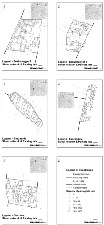
Five different micro-districts and their road networks have been analyzed in Budapest. The following five sub-urban districts were selected: Gazdagrét (GR);
KaszásdĦlĘ (KD); Pók utca (PK); Békásmegyer I (BMi); Békásmegyer II (BMii). Their locations are shown in Fig. 1. Their main statistical data i.e. size, population, area and density are shown in Table I [9].
Appropriate data collection and monitoring were necessary parts of conditional assessment. The main steps of analyzing methods applied during the examination are described below. First, data related to urban street networks were collected from OpenStreetMap.org (OSM) and they have been recorded in the Geographical Information System (GIS) database. ArcGIS software was used for data storage. This process ensured that relevant features of urban street networks, i.e. street layout, hierarchy of roads and location of one-way streets were duly recorded. Monitoring of urban street layouts was the second step. In this stage, the appropriateness of urban street network data from OSM was controlled by field surveys.
Fig. 1. Urban street network of selected sub-districts in Budapest
Table I
Main data of selected micro-districts
Sub-districts Area [km2 ] Resident population [inhab] Number of dwellings [pc] Population density [inhab/km2 ] Housing density [pc/km2 ] Number of dwellings/resident population [pc/inhab] Building period [years]
BMi 0.898 21020 9403 23416.5 10475.0 2.235 1970-89
BMii 0.589 12451 5573 21127.7 9456.7 2.234 1970-89
GR 0.426 9894 4968 23225.4 11662.0 1.992 1981-90 KD 0.333 7548 3319 22666.7 9967.0 2.274 1981-84 PK 0.704 8978 4532 12752.8 6437.5 1.981 1970-89
During the field survey the efficiency of traffic calming, the amount of parking facilities and the dimensions of cross-sections were measured. GIS database was corrected by these measurements.
In everyday transportation, one-way traffic has an influence on traffic flow. It determines usable routes of private and public transportation modes. In this paper, one (in the case of one-way street) or two (in the case of two-way street) street segments were considered between adjacent intersections. This methodology was used instead of one street segment between every neighboring intersection. Therefore, street segments have been given a direction.
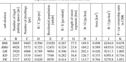
Number of pieces and types of legal parking spaces were counted with survey and satellite images (GoogleEarth). In most of the cases, the ratio of residential population and the current number of parking spaces do not reach the car ownership ratio in Central Hungary Region (CHR) (394 cars/person) [10]. A shortage of parking spaces is shown in Table II. Traffic generation points were represented by parking spaces.
As columns F and K in Table II show numbers of legal parking facilities are currently serious problem in residential areas. Likewise, it seems to be the problem to compare column D to the current National Urban Development and Construction Requirements (NUDCR) [11] in force, which requires 1 parking space per dwelling unit.
During assessment of sub-districts, it was important to analyze the potential connections of residential street networks to urban arterial roads. These arterial roads have significant tasks in traffic flow. Approximately length of these roads equals to 20% of entire street networks. Additionally, they carry on the 80% of traffic flow [12].
Therefore, the arterial roads with dense traffic appeared in microscopic models. Actual traffic conditions of arterial roads were given from Center for Budapest Transport (CBT). These roads were taking into account as exit roads from analyzed residential areas.
Table II
Important details of urban street networks
sub-districts Number of legal parking spaces [pc] Number of dwellings [pc] B / C [pc/pc] Residential population [inhab] B / E [pc/inhab] Length of street segments [km] B / G [pc/km] Area [km2 ] B / I [pc/km2 ] F / car ownership ratio in CHR
A B C D E F G H I J K
BMi 5605 9403 0.596 21020 0.267 37.5 149.5 0.898 6244.0 0.678 BMii 4028 5573 0.723 12451 0.324 23.8 169.2 0.589 6835.0 0.822 GR 3920 4968 0.789 9894 0.396 19.4 202.1 0.426 9211.3 1.005 KD 2127 3319 0.641 7548 0.282 16.8 126.7 0.333 6395.4 0.716 PK 3717 4532 0.820 8978 0.414 32.7 113.7 0.704 5279.8 1.051
2.2. Examined models
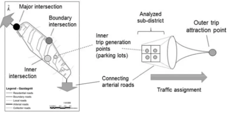
The aim of this study was searching connections between the capacity of streets, types of traffic calming methods and characteristics of the urban street layout at the whole network [13]. For this purpose, static macroscopic transportation models were used for traffic assignment. Intersections and street segments are the components of the street networks. They have a deep influence for the traffic flow and in case of interrupted oversaturated traffic conditions the regular functions of traffic flow are not clearly useable most of the time [14], [15]. In this step PTV VISUM software has been used. Earlier defined shape-files were imported from GIS database system to microscopic models in every examined case. In traffic assignment, traffic from center outwards was taken into account. Therefore, trip generation points were represented by surveyed parking spaces with their locations and capacities. Trip attraction point was determined as outer point. This outer point situated outside of the examined areas and the earlier defined arterial roads ensured connections from sub-districts to attraction point. The traffic assignment process is shown in Fig. 2.
During traffic assignment process, the street networks were loaded with the different amount of traffic. Furthermore, personal vehicles were only simulated. In practice, public transport services, pedestrian facilities and location of workplaces are impacted on traffic [16]. Volumes of generated traffic in the networks were specified as the combination of the capacity of parking spaces and the car ownership ratio in Central Hungary Region (394 cars/person). The minimum of generated traffic was 10 percent of the capacity of parking spaces, the maximum of generated traffic was equaled to the car ownership ratio relating to the population of examined urban areas. In some cases, the maximum traffic volume was higher than the car ownership ratio. At every incremental step, traffic load was 10% higher than former step until volumes of traffic loads reached the formerly defined maximum of generated traffic. The amount of traffic where mean speed was suddenly decreased and mean travel time was suddenly increased, further
intermediate values were analyzed. Generated traffic was higher in some cases than actual traffic. Time period of traffic analysis was 1 hour in the morning. This approach provides detailed picture of capacity and characteristics of traffic flow on urban street networks.
Fig. 2. Urban street layout of selected micro-districts
The traffic lanes of street sections in the macroscopic model were defined with the current street topology as mentioned earlier i.e. the number of lanes, one-way streets, applied speed and traffic calming methods. Parking spaces were modeled as inner zones in VISUM models. Intersections were determined with the Highway Capacity Manual (HCM) based. Detailed node impedance calculation was applied in node editor (ICA) module in case of VISUM models. This module ensures that the volume of traffic on loaded traffic network has an influence on turning time delays at the intersections.
The applied intersections were named based on their locations in this paper as it is shown in Fig. 2. The major intersection is an at-grade junction at the crossing of boundary roads. The generated traffic could leave the inner zones through this type of nodes. The boundary intersection is an at-grade junction at the boundary or arterial roads. The inner intersection is an at-grade junction at the traffic calming areas.
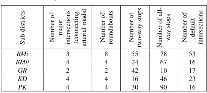
Intersections in the macroscopic models were defined as follows. Intersections of residential roads were defined as an all-way stop. Intersections of boundary and collector roads were defined as a two-way stop. Major intersections and main junctions of boundary and collector roads were defined as a roundabout, what type of intersections they have.
Streets are named based on their locations similar to intersections as it is shown in Fig. 2. The residential street is a traffic calmed street in the analyzed sub-districts. The boundary street is a street at the boundary of sub-districts. The collector street is a main street in the sub-districts. The local street is a street outside the sub-districts, and they were not taken into account during macroscopic modeling. The arterial street is a major street which ensures the connection with other parts of the settlement [17].
One direct link could be defined between two nodes only in the macroscopic model.
Therefore, the model does not contain any loop streets, and some nodes have only two arms. They were defined as default. The summary of defined intersections is shown in
Table III. Moreover, the major intersections were handled in a similar way independently their actual type (sign or signal intersection). This boundary condition was important during the analysis process. Outgoing traffic from the sub-districts was only analyzed. With these boundary conditions, the street networks of analyzed sub- districts could be comparable based on their parking facilities and residential population. Highly-detailed picture of diverse urban street layouts are given by this method.
Table III
Important details of urban street networks
Sub-districts Number of major intersections (connecting arterial roads) Number of roundabouts Number of two-way stops Number of all- way stops Number of default intersections
BMi 3 8 55 78 53
BMii 4 4 24 67 16
GR 2 2 42 10 17
KD 4 4 16 46 23
PK 4 4 30 90 16
3. Results and discussions 3.1. Morphology analysis
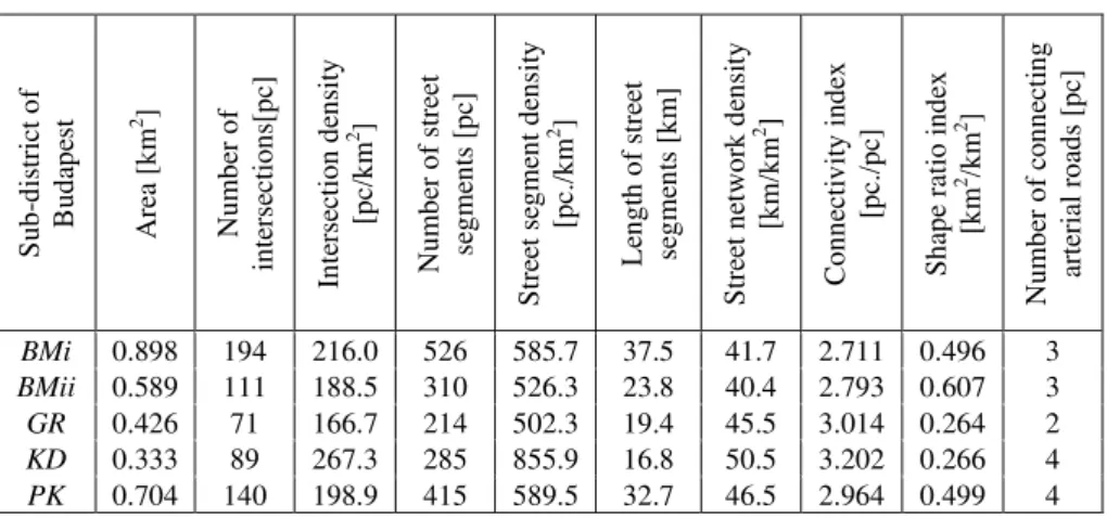
The following terms were used in the process of data analyzing. These terms have many variants and they have long term usages [18]. Street Network Density (SND) is equal to the length of street segments divided by the area of sub-district. Street Segment Density (SSD) is defined as the number of street segments divided by the area of sub- district. Intersection Density (ID) is defined as the number of intersections divided by the area of sub-district. Connectivity Index (CI) is also called as Link to node ratio. It equals to the number of street segments divided by the number of intersections. Shape Ratio Index (SRI) is defined as the area of circumscribed circle of sub-district divided by the area of sub-district. A shape of area has been characterized with this ratio index.
Besides, shape ratio of a square equals to 0.637. If this ratio is lower than 0.637, the area is oblong. Results of morphological analysis are shown in Table IV.
The analyzed sub-districts are micro-districts with residential land use. Their street patterns are similar to each other but they have differences in some characteristic terms.
Morphological results are detailed by the following paragraphs. The major differences in analyzed street networks appear with values of ID, SSD, SND and CI. Directed streets networks do not contain the banned direction. Based on originally designed street networks, they could be separated into two groups. BMi and GR are included in the first group, BMii, KD and PK are included in the second group. Because of this, the following results have significant differences. KD has the highest values of analyzed measures. This is due to the shape of micro-district. It is long and thin, and its inner
street network is dense as it is shown in Table IV. Street network of GR has contrary results. It has a rare street network based on SSD and ID. Analyzing directed networks, value of SND is similar to PK and it is higher than values of BMi and BMii. The case of CI acts similarly. It means, street network of GR is not as dense as others taking the number of directed street segments into account. But the length of street segments, the value of SND is higher than BMi and BMii. Therefore, it is denser than them. The street network values of PK are similar to BMi and GR. Taking SSD into account, the value is close to the result of BMi. Additionally, CI values are close to values of GR. Some similarities exist between the street network of BMi and BMii. Similarity is due to similar building period and their vicinity. BMi has the longest street network. BMii has the lowest SND value and values of SSD and CI are close to the value of GR.
Intersections have the highest influence on traffic flow next to the road segments.
Districts with lower CI value have fewer road paths and alternative routes. Number and location of major intersections are very important because traffic could leave the inner zones through these nodes. The proportional of intersections at the boundary roads to inner intersections is similarly important aspect. SRI shows the shape of GR and KD is oblong and the shape of BMi, BMii and PK is almost square.
Table IV
Important details of urban street networks
Sub-district of Budapest Area [km2 ] Number of intersections[pc] Intersection density [pc/km2 ] Number of street segments [pc] Street segment density [pc./km2 ] Length of street segments [km] Street network density [km/km2 ] Connectivity index [pc./pc] Shape ratio index [km2 /km2 ] Number of connecting arterial roads [pc]
BMi 0.898 194 216.0 526 585.7 37.5 41.7 2.711 0.496 3 BMii 0.589 111 188.5 310 526.3 23.8 40.4 2.793 0.607 3 GR 0.426 71 166.7 214 502.3 19.4 45.5 3.014 0.264 2 KD 0.333 89 267.3 285 855.9 16.8 50.5 3.202 0.266 4 PK 0.704 140 198.9 415 589.5 32.7 46.5 2.964 0.499 4
3.2. Results of traffic assignment Travel time and speed
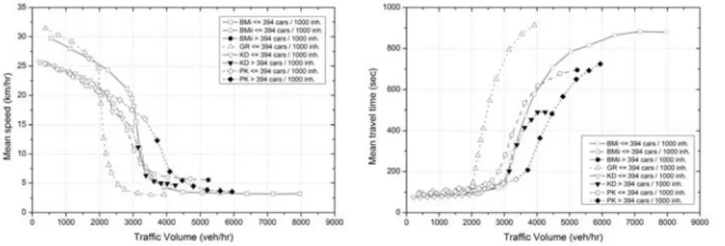
The following section contains results of the macroscopic modeling process. Time period was 1 hour in every case, and traffic volume were depended on the population of sub-districts. Travel time was measured from inner trip generation points (parking places) to outer trip attraction point in every situation as it is shown in Fig. 2. The connection between mean travel time versus traffic volume and mean speed versus traffic volume are shown in Fig. 3 and Fig. 4. In Fig. 3 the mean speed is plotted along
the y-axis and traffic volume is plotted along the x-axis. In Fig. 4 the mean travel time is plotted along the y-axis and traffic volume is plotted along the x-axis. Based on the results, the sub-districts could be separated into two groups. BMi and GR are part of the first group, and BMii, KD and PK are part of the second group. The number of major intersections has an important effect on the results and the classification. The first group has approximately 5 km/h higher mean speed than the second group with initial traffic volume. Boundary and collector streets are available from inner streets via a few intersections. Therefore, the vehicles have reached higher mean speed than in other cases. Around 2000 veh/hr in the case of GR and 3000 veh/hr in case of BMi, the mean speed is suddenly decreased and travel time is increased by the results. Outcomes are connected with the number of major intersections. Major intersections of street layouts are reached their capacity at these traffic conditions, and street networks are simultaneously oversaturated. Traffic from generated points could be reached attraction point via few inner intersections. Hence, surround traffic of intersections were interrupted. This phenomenon appeared also in BMii, KD and PK in a focused way as the case of BMi and GR.
Fig. 3. Mean speed vs. traffic volume Fig. 4 Mean travel time vs. traffic volume Results of modeling process could be explained by the number of major intersections (exits) of the sub-districts. Moreover, they have greater influence on traffic flow than the types of street segments in urban space. This could explain the unique behavior of BMii. The behavior of street network is a little bit different from KD and PK under increasing traffic volume. Simultaneously it is almost part of the first group. It has 3 major intersections similar to BMi, but its traffic assignment outcome is close to KD. The slope of the middle part graph in Fig. 3 is not as steep as BMi or GR.
Therefore, traffic volume from approximately 2500 veh/hr mean travel time is gradually increased and the mean speed is decreased. After a critical traffic volume, mean speed is constantly low in every case. Urban street networks are oversaturated, and the required space of vehicles is close to the total length of street networks.
Speed-density and slowness-speed connection
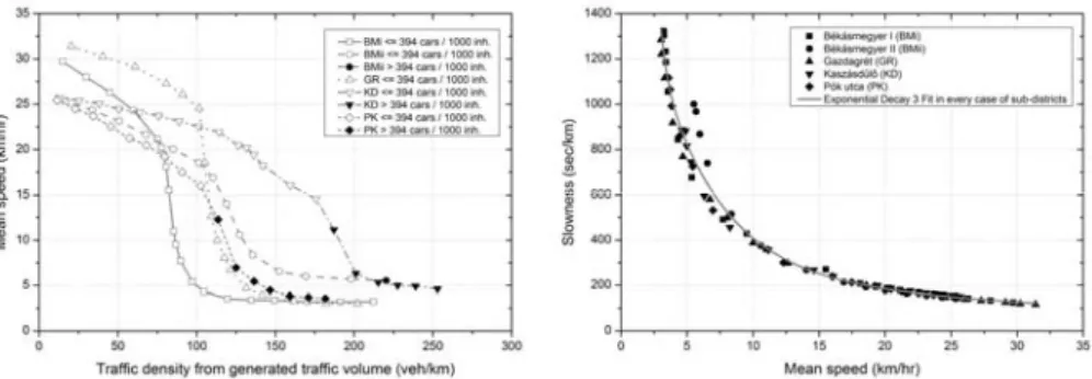
Relationship of speed and density is shown in Fig. 5. This connection is part of fundamental diagram of traffic flow. That is adequate described in case of street
segments but not for entire street network. Type and number of intersections and street segments have a great impact on the results. Further research is needed to describe the exact connection among parts of street networks.
The slowness [19] (specific travel time) equals to the change in time per unit distance [s/m] as a function of distance is defined in (1), where t is the travel time; x is the distance and w is the slowness,
( ) ( )
dx x x dt
w = . (1)
The connection between speed and slowness is shown in Fig. 6.
Fig. 5. Mean speed vs. traffic density Fig. 6. Slowness vs. mean speed
The figure shows, due to a fixed increase in speed the savings in travel time becomes smaller, the greater the value of final speed. In Fig. 4, the slowness is plotted along the y-axis and the mean speed of vehicles is plotted along the x-axis. The fitted curves as exponential decay 3 is represented with grey line. Applied form of exponential decay 3 fit (2) was the following:
3 2
1 2 3
1
0 Ae xt Ae xt Ae xt y
y= + − + − + − , (2)
where y0 is the offset; A1, A2, A3 are the amplitude; t1, t2, t3 are the decay constant. For every data, only one curve was fitted. The R-square value of this fitted curve is 0.98.
Parameters of exponential decay 3 fit are shown in Table V. It shows that data from traffic assignments and street networks of neighborhoods are similar to each other.
Points of graphs in Fig. 6 are similar to each other, they overlap one another.
Despite the fact, that layout of street networks and residential population are different.
The exponential fit has similar shape to professional literature [20]. Differences among sub-districts in travel time and speed are not detectable.
Table V
Parameters of exponential fit in case of Fig. 6
y0 value A1 value t1 value A2 value t2 value A3 value t3 value Statistics adj.R- square
-3581.18 3802.58 1153.63 1711.56 4.88 94968.1 0.49 0.978
Delay at intersections
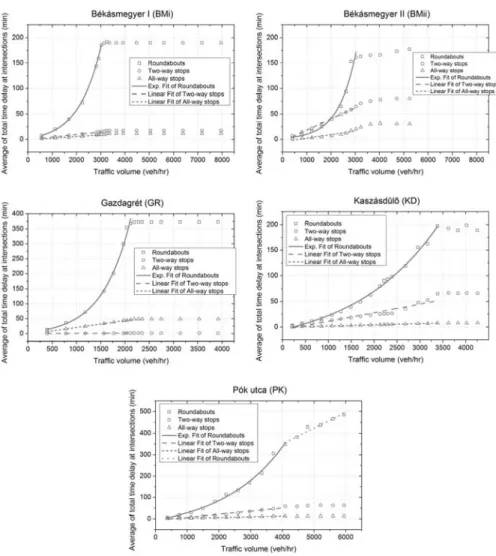
Intersections have an impact on vehicles in travel time delay. These delays depend on the type and location of intersections and the volume of traversing traffic. The mean of total time delay at one intersection was calculated by the proportion of the number of that type of intersections to total time delay at that type of intersection. Results are shown in Fig. 7. In the plotted graphs the y-axis presents the average of total time delay at intersections and the x-axis the traffic volume is assigned.
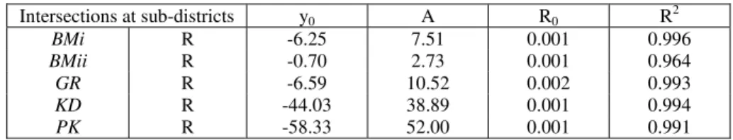
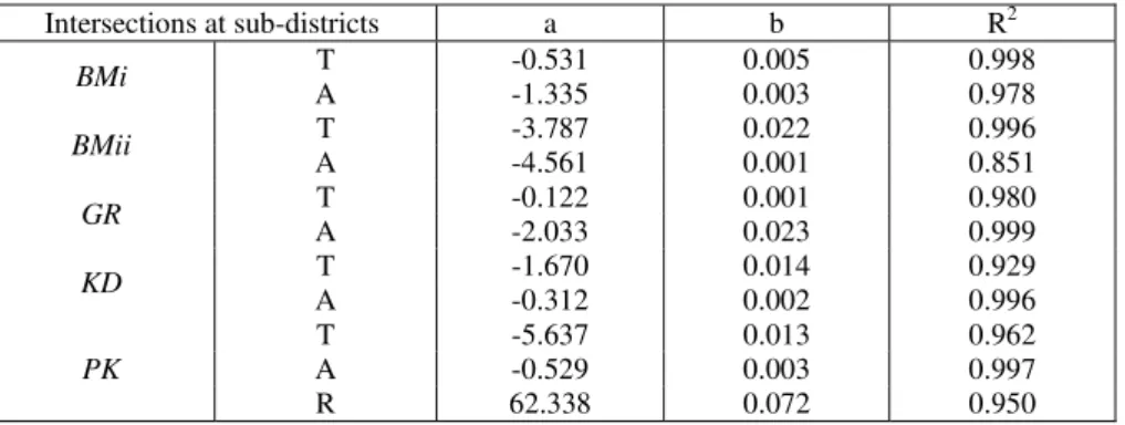
Parameters of exponential and linear fits are shown in Table VI and Table VII.
Measured points at roundabout graphs could be fitted with exponential curves, and graphs of two-way stop and all-way stop could be fitted with linear curves. Formula of used exponential fit (3), where y0 is the offset, A is the amplitude and R0 is the rate, and linear fit (4), where a is the intercept and b is the slope. Equations of fits were the following:
x AeR y
y= 0+ 0 , (3)
bx a
y= + . (4)
Values of y-axis are different in some cases. Outcomes depend on the number and location of major intersections. That could be explained by appearing traffic volume of major intersections and intersections of boundary and collector roads are higher than in case of other types of intersections but their numbers are lower than others.
Table VI
Parameters of exponential fits in case of Fig. 5, R: Roundabout Intersections at sub-districts y0 A R0 R2
BMi R -6.25 7.51 0.001 0.996
BMii R -0.70 2.73 0.001 0.964
GR R -6.59 10.52 0.002 0.993
KD R -44.03 38.89 0.001 0.994
PK R -58.33 52.00 0.001 0.991
Fig. 7. Average of total time delay at intersections vs. traffic volume
4. Conclusions
Based on given results, the traffic assignment is affected by shape of area, numbers and locations of connecting arterial roads, urban street layout and applied traffic calming systems. The aim of the examination was comparing different urban street layouts. Hence, morphological analyzes and traffic assignment was used at existing road networks of five selected micro-districts. The results of examination of street network could be summarized with following statements. Characteristic values of traffic flow could be influenced by numbers of major intersections and their locations. Their effects are stronger than street network patterns. Under increasing traffic volume, exponential
time delay exists at major intersections, and linear time delay exists at boundary and inner intersections. Slowness-speed connection represents the quality of traffic. The graph has exponential function. In the further work, theoretically, grid layout model with different shape will be used for deeper results.
Table VII
Parameters of linear fits in case of Fig. 5, T: Two-way stop; A: All-way stop; R: Roundabout
Intersections at sub-districts a b R2
BMi T -0.531 0.005 0.998
A -1.335 0.003 0.978
BMii T -3.787 0.022 0.996
A -4.561 0.001 0.851
GR T -0.122 0.001 0.980
A -2.033 0.023 0.999
KD T -1.670 0.014 0.929
A -0.312 0.002 0.996
PK
T -5.637 0.013 0.962
A -0.529 0.003 0.997
R 62.338 0.072 0.950
References
[1] Næss P. Urban form and travel behaviorௗ: Experience from a Nordic context, J. Transp.
Land Use, Vol. 5, No. 2, 2012, pp. 21–45.
[2] Schmidt K. J., Poppendieck H., Jensen K. Effects of urban structure on plant species richness in a large European city, Urban Ecosyst, Vol. 17, No. 2, 2014, pp. 427–444.
[3] Zhong C., Arisona S. M., Huang X., Batty M., Schmitt G. Detecting the dynamics of urban structure through spatial network analysis, Int. J. Geogr. Inf. Sci. Vol. 28, No. 11, 2014, pp. 2178–2199.
[4] Mátrai T., Tóth J. Comparative assessment of public bike sharing systems, Transp. Res.
Period, Vol. 14, 2016, pp. 2344–2351.
[5] Wong W., Wong S. C. Network topological effects on the macroscopic Bureau of Public Roads function, Transportmetrica A: Transport Science, Vol. 12, No. 3, 2016, pp. 272296.
[6] Sheikh A., Zadeh M., Rajabi M. A. Analyzing the effect of the street network configuration on the efficiency of an urban transportation system, Cities, Vol. 31, 2013, pp. 285–297.
[7] Miyagawa M. Hierarchical system of road networks with inward, outward, and through traffic, J. Transp. Geogr, Vol. 19, No. 4, 2011, pp. 591–595.
[8] Hegyi P. Road patterns of housing estates in Hungary, Pollack Periodica, Vol. 10, No. 1, 2015, pp. 83–92.
[9] Hungarian Central Statistical Office - Detailed Gazetteer of Hungary, https://www.ksh.hu/
apps/hntr.main?p_lang=EN, (last visited 19 December 2016).
[10] Eurostat regional yearbook 2016 edition, 2016, http://ec.europa.eu/eurostat/statistics- explained/index.php/Eurostat_regional_yearbook, (last visited 19 december 2016).
[11] National Urban Development and Construction Requirements (in Hungarian), https://net.jogtar.hu/jr/gen/hjegy_doc.cgi?docid=99700253.KOR, (last visited 19 December 2016).
[12] Jiang B. A topological pattern of urban street networksௗ: Universality and peculiarity, Physica A, Vol. 384, No. 2, 2007, pp. 647–655.
[13] Vasvári G. Affection radii of congested junctions on traffic networks, Periodica Polytechnica, Civ. Eng, Vol. 58, No. 1, 2014, pp. 87–92.
[14] Mahmassani H., Williams J. C., Herman R. Performance of urban traffic networks, In:
Transportation and Traffic Theory, N. H. Gartner, N. H. M Wilson (Eds.), Elsevier, 1987, pp. 118.
[15] Sharma H. K., Swami M., Swami B. L. Speed-flow analysis for interrupted oversaturated traffic flow with heterogeneous structure for urban roads, International Journal for Traffic and Transport Engineering, Vol. 2, No. 2, 2012, pp. 142152.
[16] Kovács Igazvölgyi Zs. Analyses of pedestrian characteristics at zebra crossings on one way roads, Pollack Periodica, Vol. 8, No. 2, 2013, pp. 67–76.
[17] Kosztolanyi-Ivan G., Koren C., Borsos A. Recognition of built-up and non-built-up areas from road scenes, Eur. Transp. Res. Rev, Vol. 8, No. 2, 2016, pp. 1–9.
[18] Knight P. L., Marshall W. E. The metrics of street network connectivity: their inconsistencies, J. Urbanism: Int. Res. on Placemaking and Urban Sustain, Vol. 8, No. 3, 2015, pp. 241–259.
[19] Leutzbach W. Introduction to the theory of traffic flow, Springer-Verlag, 1988.
[20] Koller S. Traffic engineering and transportation planning, (in Hungarian) MĦszaki Könyvkiadó, Budapest, 1986.