Experimental fitting of rotor models by using a special three-node beam element
Mate Antali
Department of Applied Mechanics Budapest University of Technology and Economics,
Budapest, 1111 Hungary Email: antali@mm.bme.hu
Denes Takacs
Department of Applied Mechanics Budapest University of Technology and Economics,
Budapest, 1111 Hungary Email: takacs@mm.bme.hu
Gabor Stepan
Department of Applied Mechanics Budapest University of Technology and Economics,
Budapest, 1111 Hungary Email: stepan@mm.bme.hu
In this paper, a special type of beam element is developed with three nodes and with only translational degrees of freedom at each node.
This element can be used effectively to build low degree-of-freedom models of rotors. The initial model from the Bernoulli theory is fitted to experimental results by nonlinear optimization. This way, we can avoid the complex modelling of contact problems between the parts of squirrel cage rotors. The procedure is demonstrated on the modelling of a machine tool spindle.
1 Introduction
In the analysis of the machine tool spindle units, it is important to consider all components of the machine (see [1] for an overview).
When simulating the milling process, it can be important to model the dynamics of the main spindle of the machine tool. Instead of a large model of the spindle with many degrees of freedom, it is efficient to create a model with a few degrees of freedom, which can be directly connected to the model of the tool and the workpiece.
One possible approach is to create the low degree-of-freedom model directly from a few beam elements (see different types of finite elements in [2], [3], [4] and [5]). For slender shafts, the Bernoulli elements can provide acceptable results, and the accu- racy of the model can be increased by using Timoshenko beam ele- ments [3, 6].
A different approach for creating a low degree-of-freedom model is the Component Mode Synthesis (CMS, see [7–9]). In this method, a detailed finite element model of the spindle is cre- ated (see e.g. [10, 11]), and then, the low degree-of-freedom model is obtained by dynamic model reduction algorithms (see [12] for and overview of the different methods). The resulting model and the original detailed model has approximately the same dynamics considering the first few vibration modes.
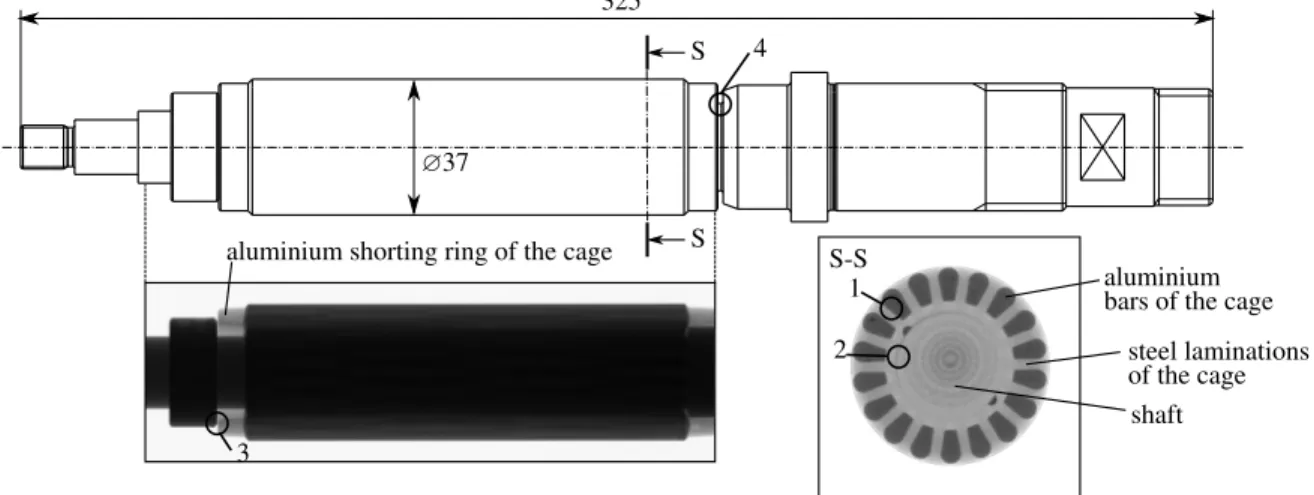
In both cases, it is necessary to know not only the detailed geometry of the shaft but the stiffness properties of the material, as well. This leads to problems in case of spindles with a squirrel-cage rotor, because the contact between the different parts significantly
modifies the stiffness of the rotor (see Fig. 1). By neglecting the effect of the contact on the stiffness, the finite element models pre- dict much higher stiffness than the measured values. For example, the finite element model of the rotor in Fig. 1 provides natural fre- quencies which are 50-70% higher compared to the measurements if fixed connections are assumed at the contacts. A possible solu- tion would be the detailed modelling of the contacts inside the rotor but many information about the contacts is not available. Hence, a reliable model of a squirrel cage rotor can hardly be created with- out measurements. As if it is necessary to modify the model to the measured data, the usage of the detailed model and CMS reduction is not efficient any more.
In this paper, we create the approximate low degree-of- freedom model directly, and then, this model is modified iteratively to fit the measured dynamical properties. The analysis of this paper is restricted to the 1D lateral vibrations of rotors, but the iteration can be applied to 3D models including longitudinal and torsional vibrations and gyroscopic effects, as well. In the model, we use a new type of beam element, which contains 3 nodes with a single translational degree of freedom at each node. Beam elements with three nodes can be found in the literature (see [13,14]), but omitting the rotational degrees of freedom has advantages at the numerical fitting.
The proposed lumped parameter model is not a finite element model in the classical sense because the elements overlap each other at the adjacent sections. Instead, the procedure leads to a special finite segment model (see [15] for a different finite segment model or [16] for the classification of the different models). Still, we refer to the building block of the model as a ”beam element”.
The structure of the paper is the following: In Section 2, the general 3-node element is presented, and the minimal set of param- eters is derived. In Section 3, the Bernoulli beam theory is applied to the 3-node element, and the resulting element is demonstrated on examples. This approximate model serves as an initial condition of the numerical iteration presented in Section 4, where nonlinear op- timization methods are utilized to fit the model to the measured nat- ural frequencies. In Section 5, the developed methods are demon-
strated on two case studies: First, a theoretical example of a simple beam is shown for validation of the method. After that, the fitting of the model is shown for the spindle in Fig. 1.
2 General beam element with 3 translational nodes
When modelling the 1D transversal vibrations of a beam, the usual choice is the 2-node beam element with a translational and a rotational degree of freedom at both nodes. However, we want to create a model with the simplest possible structure, therefore, we restrict the model to the translational degrees of freedom. As a side- effect, minimumthreenodes are required to model the bending of the beam (see Fig. 2). In addition to its simplicity, this construction helps to avoid some numerical complications at the fitting. By us- ing the usual beam elements, there are components in the stiffness and mass matrices with different dimensions, which leads to badly conditioned optimizing problems. Moreover, the lumped mass ma- trix of the usual beam element is singular (see [17] p. 242 or [18], p. 540). By omitting of the rotational degrees of freedom, these problems do not occur.
In this section, we derive the structure and the properties of the stiffness and mass matrices without considering the actual geometry and material properties of the spindle. In Section 3, the necessary parameters are determined by using the Bernoulli beam theory.
2.1 Structure of the stiffness matrix of a general element The axial position of the three nodes are denoted byx1,x2,x3, the displacements of the nodes are denoted byw1,w2,w3, and thus, the element position and displacement vectors are
xe=
x1 x2 x3
, we=
w1 w2 w3
(1)
(see Fig. 2). The length of the element is denoted byL=x3−x1 and the dimensionless position λ∈[−1,1]of the middle node is defined by
λ=2x2−(x1+x3)
L . (2)
In the special caseλ=0, the middle node is located exactly in the middle of the element.
Consider the stiffness matrix of the element in the form
Ke=
k11 k12 k13
k12 k22 k23
k13 k23 k33
. (3)
The number of the independent parameters of the stiffness matrix is reduced by the homogeneous static equilibrium equations of the element. Consider the elemental displacements
e1=
1 0 0
, e2=
0 1 0
, e3=
0 0 1
(4) of the nodes (see Fig. 3).
For these displacements, the equilibrium equations can be written into the form
etTKee1=0, eTtKee2=0, etTKee3=0,
eTrKee1=0, eTrKee2=0, eTrKee3=0, (5)
where the vectors et=
1 1 1
, er=
L 2(λ+1)
0
L 2(λ−1)
, (6) correspond to the coefficients of the equilibrium equations related to the forces and the moments, respectively. The equations (5) leads to
1 1 1 0 0 0
0 1 0 1 1 0
0 0 1 0 1 1
(λ+1) 0 (λ−1)0 0 0 0 (λ+1) 0 0(λ−1) 0
0 0 (λ+1)0 0 (λ−1)
·
k11
k12
k13 k22
k23
k33
=
0 0 0 0 0 0
. (7)
The rank of the coefficient matrix is 5, thus, only one component of the stiffness matrix can be chosen independently. Let us introduce the notationk22=k, and then, by solving (7), the stiffness matrix (8) becomes
Ke=k·
(1−λ)2 4
−(1−λ) 2
(1−λ)(1+λ) 4
−(1−λ)
2 1 −(1+λ)2
(1−λ)(1+λ) 4
−(1+λ) 2
(1+λ)2 4
. (8)
In the special caseλ=0 of an element with equally spaced nodes, the stiffness matrix becomes
Ke=k·
1/4 −1/2 1/4
−1/2 1 −1/2 1/4 −1/2 1/4
. (9)
Note, that a similar analysis can be carried out for the usual 2-node beam element with translational and rotational degrees of freedom. It can be shown that for that type of element,twoparam- eters of the stiffness matrix can be chosen independently, related to the bending and the shear of the element. The presence of these two parameters with different dimensions and magnitudes leads to complications at the efficient numerical fitting. A possible solution could be the fixing of these two parameters to each other (by using e.g. the Bernoulli beam theory), but then, more degrees of free- dom would be necessary for the same number of free parameters.
These properties show the advantage of the proposed model with no rotational degrees of freedom.
2.2 Mass matrix and effective model
The simplest relevant form of the mass matrix can be written into the diagonal form
Me=
m1 0 0 0 m2 0 0 0 m3
, (10)
wherem1,m2andm3are the lumped masses at the nodes. Finally, the free vibrations of a single element are described by the equation of motion
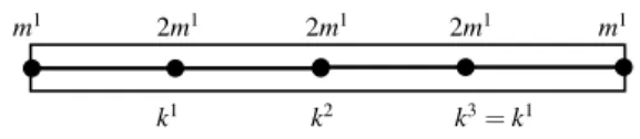
Mew¨e+Kewe=0. (11) The resulting equation is equivalent to the effective model contain- ing three mass points connected by massless rigid bars (see Fig.
4). The appropriate stiffness can be provided by a single torsional spring with a torsional stiffness
kt=L2(1−λ)2(1+λ)2
16 ·k. (12)
aluminium
shaft
steel laminations aluminium shorting ring of the cage
bars of the cage of the cage
S S-S
S 325
1 2
3
4
∅37
Fig. 1. The analysed spindle with a squirrel cage mounted on the shaft. Top panel: drawing of the spindle of the tested milling machine.
Bottom-left panel: CT image of the spindle in a longitudinal section. Bottom-left panel: CT image of the spindle in a transversal section. The numbered circles denote the modelling challenges. 1: contact between the aluminium and steel parts of the cage. 2: contact between the cage and the shaft. 3: contact between the cage and the fixing ring. 4: contact between the cage and the edge of the shaft.
w1 w2 w3
x1 x2 x3
L L(1+λ)/2
Fig. 2. Sketch of the 3-node general beam element with transla- tional degrees of freedom.
e1 e2 e3
Fig. 3. The nodal forces creating the elemental displacements. The equilibrium of these force systems has to be ensured in the stiffness matrix.
Hence, all four parameters of the element (k,m1,m2,m3) of the elements are related to simple physical meaning of this effective model.
Note, that more general structures of mass matrix could be also introduced. It is possible to connect lumped mass moments of inertia either to the nodes or to the midpoints of the sections. In both cases, the rotations can be approximated from quadratic and linear interpolation of the nodal displacements, respectively. This procedure results in the appearance of additional non-zero elements in the mass matrix (10).
2.3 Connection of the elements
When more of these 3-node elements are connected to model a beam,twonodes of the adjacent elements have to be coupled (see Fig. 5). This is necessary to transmit bending moment between the elements because the nodes do not have a rotational degree of freedom.
m1 m2 m3 kt
Fig. 4. The effective model of the 3-node beam element: three mass points connected by rigid massless bars and a torsional spring.
element 1 element 2 element 3 assembled model
Fig. 5. Connection of the 3-node beam elements.
The resulting stiffness and mass matrices of the model have the form
K=
∗ ∗ ∗0 0
∗ ∗ ∗ ∗0
∗ ∗ ∗ ∗ ∗ 0∗ ∗ ∗ ∗ 0 0∗ ∗ ∗
, M=
∗0 0 0 0 0∗0 0 0 0 0∗0 0 0 0 0∗0 0 0 0 0∗
, (13)
respectively, where the symbol ∗denotes the nonzero elements.
That is, the stiffness matrix of the model is penta-diagonal and the mass matrix is diagonal. In case ofnnodes, the model has a stiff- ness matrix withn−2 independent parameters and a mass matrix with nindependent parameters. These parameters are related to those of an effective model from bars, mass points and torsional springs (see Figure 6). In that sense, the presented model leads to a finite segment modelwhere each element is related to two segments (sections).
3 Initial assumption by using the Bernoulli theory
At the simplest case of the usual 2-node beam elements, the element matrices are derived by using the Bernoulli beam theory,
Fig. 6. Effective model of several connected elements.
which provides a good approximation for slender beams. This the- ory can be applied to the 3-node beam element of Section 3, as well.
Therefore, the parameters of (9) and (10) can be determined from the physical properties of the rotor. From the resulting Bernoulli elements, an approximate model can be built, which will serve as initial values for the numerical iteration presented in Section 4.
3.1 Derivation of the element matrices
To get the lateral displacement functionw(x)of the element, a second-order interpolation is used between the three nodes in the form
w(ξ) =aξ2+bξ+c=N1(ξ)w1+N2(ξ)w2+N3(ξ)w3, (14) whereξ=2x/L−1 is the dimensionless coordinate along the el- ement andN1(ξ),N2(ξ),N3(ξ)are the shape functions. From the boundary conditions
w(−1) =w1, w(λ) =w2, w(1) =w3, (15) the vector of the shape functions becomes
N(ξ) =
N1(ξ) N2(ξ) N3(ξ)
=
(ξ−1)(ξ−λ) 2(λ+1)
−(1−λ)(1+λ)(ξ−1)(ξ+1)
(ξ+1)(ξ−λ) 2(λ−1)
. (16)
By using the Bernoulli beam theory, we consider the potential energy from bending in the form
U=1 2
Z x3
x1 IE w00(x)2dx=1
2wTeKewe, (17) whereIis the area moment of inertia of the cross-section,Eis the elastic modulus andw00(x)is the second derivative ofwwith respect to the coordinatex. Finally, the stiffness matrix of the element is given by
Ke=IE Z1
−1
d2N(ξ)
dξ2 ·d2NT(ξ) dξ2 ·L
2dξ. (18)
The result of the integration leads to a stiffness matrix in the form (8) with
k= 32I1E1(1+λ) +32I2E2(1−λ)
(1−λ)2(1+λ)2L3 , (19) whereE1,E2andI1,I2are the properties of the two sections of the element. In the special case of thesymmetric element, that is, when λ=0,E1=E2=EandI1=I2=I, we getk=64IE/L3and (8) becomes
Ke=IE L3·
16 −32 16
−32 64 −32 16 −32 16
. (20) If the mass of both sections of the elements are divided into two equal parts at the nodes of the sections, the mass matrix (10) becomes
Me=
A1E1L(1+λ)
2 0 0
0 A1E1L(1+λ)+A2 2E2L(1−λ) 0
0 0 A2E2L(1−λ)2
. (21) One could also create a consistent mass matrix based on the shape functions (16), but we focus on the lumped mass matrix according to (10).
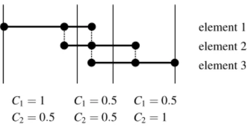
element 1 element 2 element 3
C1=1 C2=0.5
C1=0.5 C2=0.5
C1=0.5 C2=1
Fig. 7. The integration ranges of the 3-node Bernoulli elements.
The overlapping sections are divided at their midpoints.
n 1 3 5 7 15 25 55
∆wmax(%) 66.67 11.11 2.79 0.96 0.19 0.05 0.02 Table 1. The relative error of the maximal deflectionwmax in the model.
3.2 Connection of Bernoulli elements
When several 3-node beam elements are connected in the model, the sections of the elements overlap each other (see Fig.
7. To avoid the overlapping in the integration, the endpoints of the integral (18) have to be modified. To preserve the symmetry of the element, the integration domains are defined by the midpoints be- tween the nodes (see Fig. 7).
As the integrand of (18) is constant, the modification of the endpoints of the integral leads to the element stiffness
k∗=C1·32I1E1(1+λ) +C2·32I2E2(1−λ)
(1−λ)2(1+λ)2L3 , (22) where
C1=
(1 for an element at the ”left” end of the beam, 0.5 otherwise,
C2=
(1 for an element at the ”right” end of the beam, 0.5 otherwise.
(23)
In the special case of a single element,C1=C2=1, and (22) leads to (19).
3.3 Validation examples
The validation of the 3-node Bernoulli element given by (8), (19) and (21) is presented by a simple double cantilever beam (see Figs. 8 and 9). In both example, the length of the beam is 1 m, it has a circular cross-section with a diameter of 30 mm, and it is made of steel. In the first example (see Fig. 8), the beam is subjected to a steady-state distributed load with a magnitude ofp=10 kN/m. The analytical solution for the maximum deflection iswmax≈16.4 mm.
Let us model the beam withnof the 3-node beam elements, which leads tonfree and 2 fixed degrees of freedom (DoFs). The relative errors of the maximal deflection of the beam in this model can be seen in Table 1 for different values ofn. For the increasing number of elements, the relative error tends to zero; the conver- gence is relatively slow due to the second-order interpolation.
In the second example, the angular frequencies of the free vi- brations of the beam is analysed (see Fig. 9). The values of the first three angular frequencies areα1≈375 1/s,α2≈1500 1/s and α3≈3373 1/s. Table 2 shows the relative error of the frequencies computed from the model for different values ofn. By increasing the number of the elements, the relative errors tend to zero.
wmax
p
Fig. 8. Validation example 1: deflection of a double cantilever beam subjected to a constant distributed load.
α3 α2 α1
Fig. 9. Validation example 2: free vibrations of a double cantilever beam.
n 1 3 5 7 15 25 55
∆α1(%) 14.63 3.97 0.56 0.05 0.16 0.08 0.02
∆α2(%) – 0.73 0.35 0.90 0.67 0.34 0.09
∆α3(%) – 31.20 7.77 4.11 1.60 0.77 0.20 Table 2. The relative error of the first three natural angular frequen- cies in the model.
4 Numerical fitting
The mass distribution of a shaft is not affected by the contact problems mentioned in Section 1. Therefore, the lumped mass of the elements are kept fixed and only the stiffness valueskiare mod- ified by the algorithm to achieve a more accurate model than the Bernoulli approximation of Section 3.
4.1 The nonlinear problem
Assume thatmmeasured natural frequencies of the shaft are available, which are denoted by ˜f1. . .f˜m. The fitting of the stiffness values can be performed by different arrangements of supporting the shaft. We chose the case ofno support, which is approximated in the measurements by suspending the shaft by a thin rubber band (see Fig. 11). In case of no support, the first two natural frequencies are theoretically zero, which correspond to the rigid body motion of the shaft. In the measurements, these motions correspond to the low-frequency swinging and bouncing of the shaft on the rubber band, which can be clearly separated from the real natural frequen- cies by an appropriate filter.
Let us consider the model of the shaft withnelements. Then, the vector of the stiffness values is denoted by
k:= [ki] = [k1,k2, . . .kn]. (24) The task of the iteration is modifying these stiffness values to fit the model to the measurements. The mass matrixMof the model is composed from the elementary matrices (21), and the stiffness matrixKis computed from (8) by using the stiffness vectork. Then, the natural frequencies of the model satisfies
det
K(k)−fl2M
=0, l=1. . .n. (25) As the model withnelements hasn+2 degrees of freedom, and there are 2 rigid body motion modes, the model providesnnatural frequencies.
To fit the model to the measured frequencies, the system fl(k) =f˜l, l=1. . .min(n,m). (26)
of nonlinear variables should be solved. In case ofn=m, the sys- tem (26) has usually countably many solutions. In case ofn>m, there are usually continuously many solutions of (26). In case of n<m, the system has no solution in the general case. That is, the element numbernis required to be larger or equal to the number of measured frequencies to have the possibility to accurately fit the frequencies of the model.
The system (26) is solved by the minimization of the cost func- tion
F(k):=
min(n,m)
∑
l=1
fl(k)−f˜l
2
. (27)
The solutions of (26) correspond to the global minima of (27) with F(k) =0. In case ofn=m, countably many isolated global minima can be found, which can be reached by nonlinear optimization tech- niques. In case ofn>m, we have more than necessary parameters, and there are continuously many global minima withF(k) =0. In this case, the definition (27) can be extended by further terms to include more information about the model (see e.g. (43)).
4.2 The line search algorithm
In the algorithm, the initial stiffness values are given by the values from the Bernoulli element (see (9)),
k0=k∗:= [k∗1,k∗2, . . .k∗n]. (28) The iteration is performed in the form
kj+1=kj+βjpj, (29) wherepj is the descent direction andβj is the step length. For a positive definite functionF, the descent direction can be chosen effectively by Newton’s method in the form
pj=−
∇2F(kj)−1
·∇F(kj), (30) where∇F(kj)is the gradient and∇2F(kj)is the Hessian ofFat kj (see [19], p. 31). IfF is not positive definite then the descent direction can be set simply to the steepest gradient
pj=−∇F(kj). (31)
For the function (27), we apply the combination of the two methods:
the Newton method (30) is applied for the points with a positive definite Hessian, and the gradient method (31) is chosen otherwise.
Hence, the effectiveness of the Newton method and the robustness of the gradient method are both utilised.
During the iteration, it is essential to preserve the positivity of the stiffness valueskij, which is not just an obvious physical re- quirement, but it is necessary for the computation of the natural frequencies at (25), as well. Therefore, in each step, we limit the relative change of the stiffness values by
kij+1−kij
≤c1kij, (32) where 0<c1<1. By substituting (29) into (32), we get
|βjpij| ≤c1kij, (33) which leads to
βj≤c1·min
i∈[1,n](kij/|pij|). (34)
The value of the step lengthβjis computed by a further itera- tion in each step, which is denoted byβj,h. In case of the steepest
gradient method (31), the initial value of the iteration is chosen to the maximum allowed value by (34):
βj,0=c1·min
i∈[1,n](kij/|pij|). (35)
In case of Newton’s method (30), the initial step length is computed by
βj,0=min
1,c1· min
i∈[1,n](kij/|pij|)
, (36)
which increases the robustness of Newton’s method. The appro- priate value of the step lengthβj is computed by the line search method by using the Armijo condition (see [19], p. 33). That is, the step length is reduced by
βj,h+1=c2βj,h (37)
with 0<c2<1 until the condition
F(kj+βj,hpj)≤F(kj) +c3·βj,h·
pj,∇F(kj) (38) is satisfied with 0<c3<1. The properties of the iteration are mod- ified by the numerical constantsc1,c2andc3. If the iteration con- verges then the limit point is denoted by
k∞:= lim
j→∞kj. (39)
There is no exact procedure for choosing the numerical con- stantsc1,c2andc3, but some guidelines can be provided. The in- crease ofc1 close to 1 speeds up the iteration, but makes it less robust in the sense that in this case, the iteration may converge to a minimum being quite far from the initial point. The increase ofc2
slows down the internal iteration of the line search method, but in the meantime, the largeβvalues speed up the main iteration cycle.
The increase ofc3slows down both iteration cycles but it increases the robustness of the iteration in the sense of finding a closest min- imum. In the applications, the values can be chosen by trial and error based on the consideration of these factors.
4.3 Robustness of the solution and random search
It was already mentioned that even in the casen=m, there can be not a single solution for (26), but many other isolated solutions can occur, too. Moreover, the cost function (27) can have not only global minima but local minima, as well. Consequently, the iter- ation starting from the initial value (28) does not necessarily con- verge to the solution which we expect. The idea is to increase the robustness of the solution, is not computing just a single iteration fromk0=k∗ but computing a bunch of solutions from randomly chosen points in the neighbourhood ofk∗.
For that purpose, let us define the distance D(k0,k∗):= max
i∈[1,n] max k∗i ki0,k0i
k∗i
!!
−1. (40) That is, this distance provides the maximum ratio between the cor- responding stiffness values of the vectors. Moreover, the resulting value is reduced by 1 to get the identityD(k,k)≡0. By using the distance function (40), several initial pointsk0are chosen from the set defined by
D(k0,k∗)<Dmax. (41) The parameterDmax is chosen according to the reliability of the initial guess (28) from the Bernoulli theory. As the algorithm is planned to fit low degree-of-freedom models, thousands of itera- tions can be computed in a few minutes by using e.g. a uniform
m1 2m1 2m1 2m1 m1
k1 k2 k3=k1
Fig. 10. Model of a single cylindrical beam (see Subsection 5.1.
k0 k1 k2 k3 k∞
k1=k3[N/mm] 3.054 4.393 4.977 5.041 5.042 k2[N/mm] 2.036 2.540 2.528 2.524 2.524 F(k)(normed) 7·10−3 6·10−4 5·10−6 6·10−10 ≈0 Table 3. The iteration of the model in Fig. 10. The parameters of the iteration arec1=0.5,c2=0.6,c3=0.1.
random distribution in the set (41). Hence, it is possible to find the solutions with small basins of attraction.
The function (40) can be used for measuring the deviation of the converged parameter setk∞ from the initial guessk∗ of the Bernoulli theory. This provides an efficient measure to find the ap- propriate solution, which is probably not too far from the initial guessk∗.
5 Case studies
5.1 Fitting to the analytical frequencies of a cylindrical beam First, the algorithm is demonstrated on an example where the model is fitted not to measured data but to the analytically com- puted frequencies of a beam. Consider the 1 m long cylindrical beam which was already analysed in Subsection 3.3. Withoutany supports, the analytical natural frequencies can be computed by us- ing e.g. the Rayleigh-Krulov functions (see [20], p. 205). Assume that we have information about the first two natural frequencies, which are
f˜1=134.7 Hz, f˜2=372.8 Hz, (42) that is,m=2. Consider a model built fromn=3 elements, where the distances between the nodes are equal (see Fig. 10).
From (21), the lumped masses are m1=m5=0.689 kg and m2=m3=m4=2m1. From (22), the initial guess for the stiff- ness values isk∗1=k∗3=3.054 N/mm andk∗2=2.036 N/mm.
From these data, the initial natural frequencies of the model are f1=116.5 Hz andf2=290.1 Hz.
Asn>m, the cost function (27) can be extended by additional information about the model. Due to thesymmetryof the beam, we restrictk1=k3, thus,Fbecomes
F(k) = f1(k)−f˜1
2
+ f2(k)−f˜2
2
+ k1−k3
2
. (43)
By applying the algorithm from Subsection 4.2 starting fromk0= k∗, the iteration converges in a few steps (see Tab. 3). The iteration can fit the model accurately to the analytical frequencies (42). The distance between the solution and the initial guess isD(k∗,k∞)≈ 0.65.
In case of such a simple system, the appropriate stiffness val- ues of the model can be expressed explicitly, as well, and we get
k1∞= 4
3·(2πf˜2)2m1, k2∞= 16 ˜f2−12 ˜f1
4 ˜f2−9 ˜f1 ·(2πf˜1)2m1, (44) which leads to the same results as those in Tab. 3. By the algo- rithm in Subsection 4.3, we do not find any further solution, as it is expected from the explicit formulae (44).
Fig. 11. Suspension of the rotor by a rubber rope for the measure- ment of the natural frequencies. The frequency response functions between different points of the rotor (denoted by numbers) were mea- sured by accelerometers and a modal hammer.
measured frequencies f˜1 f˜2 f˜3 f˜4
average [Hz] 1063 2921 5183 7274 uncertainty [Hz] ±10 ±40 ±28 ±38
Table 4. The measured frequencies of the spindle shaft (see Fig.11) and the frequencies of the initial model. The uncertainty of the mea- sured frequencies are given at the confidence level of 95%.
m1
k1
m2 m3 m4 m5 m6
k2 k3 k4
Fig. 12. Model 2.
5.2 Fitting to the measured frequencies of a spindle
Consider the spindle shaft presented in Fig. 1. The free vi- brations are measured by suspending the rotor to a rubber rope (see Fig. 11). A set of measurement points were selected on the surface of the rotor, and the frequency response functions were measured between these point by using accelerometers and a modal hammer.
Therefore, not only the natural frequencies were determined but we obtained the mode shapes, as well, which will be used for further analysis. The measured frequencies are shown in Tab. 4.
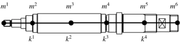
The model is created by usingn=4 3-node elements (see Fig.
12). The cage is located betweenx2andx4. The loci and the masses of the nodes are computed from the measured geometry and from the distribution of the steel and aluminium parts of the cage (see Fig. 1), which can be seen in Tab. 5.
The initial stiffnessk∗is computed from (9), where the diam- eters of the shaft are averaged along the sections. This leads to the
x1 x2 x3 x4 x5 x6
0 mm 41 mm 115 mm 190 mm 264 mm 325 mm
m1 m2 m3 m4 m5 m6
28 g 253 g 449 g 502 g 453 g 175 g
Table 5. Loci and masses of the model in Fig. 12. The overall mass of the rotor is 1860 g, which value is validated by a scale. The mass values are considered reliable and the stiffness values are modified to fit the model to the measured freqencies.
initial model frequencies f1 f2 f3 f4
[Hz] 1703 3962 5790 11513
Table 6. Initial frequencies of the model .The frequencies are com- puted from the initial stiffness valuesk∗(see Tab. 7).
1e-09 1e-08 1e-07 1e-06 1e-05 0.0001 0.001 0.01 0.1 1 10
0 5 10 15 20 25 30 35 40 45 50
costfunctionF(x)
iteration number j
Fig. 13. Reduction of the cost function during the iteration starting fromk0=k∗.
values in the first row of Tab. 7, which leads to the frequencies f1. . .f4in Tab. 6. These initial values are significantly higher than the measured frequencies ˜f1. . .f˜4 (see Tab. 4), which is probably caused by the non-modelled contact stiffness at the cage (see Fig.
1). Asn=m=4, the cost function (27) is calculated by F(k) =
4
∑
l=1
fl(k)−f˜l2
. (45)
By computing the algorithm of Subsection 4.2 fromk0=k∗, the procedure converges in about 50 iterations (see Figs. 13-14).
It can be seen from the diagrams that after about 40 steps of slow convergence, the iteration reaches the positive definite region ofF, and the switching to the Newton method speeds up the convergence.
However, by switching to the Newton method earlier, the iteration would not converge. The iteration parameters are chosen toc1= 0.5,c2=0.6,c3=0.1. Test computations show that the solution and the necessary number of iteration steps is not sensitive to the choice of the parametersc1. . .c3of the line search method. At the end of the iteration, we get the stiffness valueskI∞(see the second row of Tab. 7).
To ensure the robustness of the solution, let us start dif- ferent trajectories from randomly chosen initial points k0 with D(k0,k∗)<3 (see Subsection 4.3). During this computation, we find 12 global minima withF(k) =0. Let us sort these solutions
0 50 100 150 200 250 300
0 5 10 15 20 25 30 35 40 45 50
stiffnessvalues[N/mm]
iteration number j
k1 k2 k3 k4
Fig. 14. Convergence of the stiffness values during the iteration starting fromk0=k∗.
[N/mm] k1 k2 k3 k4 D(k∗,k∞) k∗ 272.1 159.5 152.6 246.4
kI∞ 107.9 90.3 49.3 230.3 2.097
kII∞ 90.1 368.2 46.2 72.0 2.420 kIII∞ 76.2 440.3 46.0 71.2 2.573 kIV∞ 55.1 31.8 141.9 445.3 4.023
Table 7. Solutions found by iterations started from randomly chosen points in the vicinity ofk∗of the Bernoulli model. From the 12 solu- tions, the ones are listed which are close tok∗in the sense of the distanceD.
kI∞. . .kX II∞ by the distance from thek∗, that is, let
D(k∗,kI∞)<· · ·<D(k∗,kX II∞ ). (46) From these 12 solution, the smallest distance isD(k∗,kI∞) =2.097 and the largest distance isD(k∗,kX II∞ ) =12.79. The closest four solutions are listed in Tab. 7.
Note that all the solutionskI∞. . .kX II∞ satisfy the equations (26), that is, the first four natural frequencies of the model is fitted to the measured frequencies forall these 12 parameter sets. In general, it is not trivial to find the most relevant solution. If the stiffness values k∗from the Bernoulli model are considered a good approximation then we can choose the solution which is the closest tok∗ in the sense of the distanceD. In this case study, this closest setkI∞ is the same as the result of the single iteration fromk0=k∗(see Figs.
13-14), but this coincidence is not necessary.
The choice ofkI∞can be validated by physical requirements of the stiffness values:
1. The values of k1, k2 and k3 of the solution k∞ should be smallerthan those ofk∗, because the effect of contacts at the cage is not considered when calculating the initial stiffness val- ues.
2. The valuek4of the solutionk∞should becloseto that ofk∗, because in the absence of the contact problem, the Bernoulli model gives a good approximation.
It can be checked thatkI∞satisfies these two requirements, but the other solutions do not satisfy both of them (see e.g. kII∞−kIV∞ in Tab. 7).
0 50 100 150 200 250 300
x [mm]
0
measured kI∞
kII∞ kIV∞
Fig. 15. Comparison of thefirstmode shape of the fitted models and the measured mode shape.
0 50 100 150 200 250 300
x [mm]
0
measured kIV∞
kII∞
kI∞
Fig. 16. Comparison of thesecondmode shape of the fitted models and the measured mode shape
Although the models are fitted to the measurements by using only the natural frequencies, the fitted solution can be validated by comparing the mode shapes of the models and those of the mea- surements. The comparison of the first two mode shapes can be seen in Figs. 15-16. From the models of Tab. 7, only the parameter setskI∞,kII∞andkIV∞ are showed in these figures, because the mode shapes ofkII∞ andkIII∞ are very close to each other. It can be seen that the solutionkI∞shows good agreement with the measurements, while the other solutions have larger deviations. This comparison also shows the validity of the choice ofkI∞.
By using the measured mode shapes directly, as well, we could fit the model with more degrees of freedom (n>m). To achieve that, an appropriate norm should be chosen to measure the differ- ence between the mode shapes. Then, the cost function should be extended by terms requiring that the mode shapes of the model and the measurement are close to each other.
6 Conclusion
For modelling the dynamics of rotors, a three-node beam ele- ment was introduced with a single translational degree of freedom.
The stiffness matrix of this kind of element can be expressed by a single stiffness parameter. By connecting a few of these elements, a low degree-of-freedom model of rotors was created, which avoids
some numerical complications when fitting the model to measured natural frequencies. By combining and customizing different line search methods of nonlinear optimization, an iteration process was introduced. The initial model of the iteration was computed by the Bernoulli element. Conditions were introduced to choose the rel- evant model from the several optima of the iteration. The method was demonstrated on a machine tool spindle unit. By the numeri- cal fitting, the modelling problems caused by the contact between the parts of the squirrel cage rotor were avoided. This method can be used effectively for creating the low degree-of-freedom models of spindles, and these models can be connected easily to the mod- els of the bearings and the machining process. The need for such connected models are represented, for examples, in [21] and [22].
Acknowledgements
We thank to Akos Miklos from the Budapest University of Technology and Economics for the comments on the finite element model. We thank to Gabor Porempovics from the Budapest Univer- sity of Technology and Economics for creating the detailed CAD model of the spindle. We thank to Istvan Kozma from the Szechenyi Istvan University for the CT visualisation of the spindle.
The research leading to these results has received funding from the European Research Council under the European Union’s Seventh Framework Programme (FP/2007-2013) / ERC Advanced Grant Agreement n. 340889.
References
[1] Abele, E., Altintas, Y., and Brecher, C., 2010. “Machine tool spindle units”. CIRP Annals - Manufacturing Technology, 59(2), pp. 781–802.
[2] Nelson, H. D., and McVaugh, J. M., 1976. “The Dynamics of Rotor-Bearing Systems Using Finite Elements”.Journal of Engineering for Industry,98(2), pp. 593–600.
[3] Cao, Y., and Altintas, Y., 2004. “A General Method for the Modeling of Spindle-Bearing Systems”.Journal of Mechani- cal Design,126(6), pp. 1089–1104.
[4] Gagnol, V., Bouzgarrou, B. C., Ray, P., and Barra, C., 2007.
“Stability-Based Spindle Design Optimization”. Journal of Manufacturing Science and Engineering, 129(2), pp. 407–
415.
[5] Rantatalo, M., Aidanp¨a¨a, J.-O., G¨oransson, B., and Norman, P., 2007. “Milling machine spindle analysis using FEM and non-contact spindle excitation and response measurement”.
International Journal of Machine Tools and Manufacture, 47(7-8), pp. 1034–1045.
[6] Thomas, D., Wilson, J., and Wilson, R., 1973. “Timoshenko beam finite elements”.Journal of Sound and Vibration,31(3), pp. 315–330.
[7] Nelson, H. D., Meacham, W. L., Fleming, D. P., and Kascak, A. F., 1983. “Nonlinear analysis of rotor-bearing systems us- ing component mode synthesis”. Journal of Engineering for Power,105(3), pp. 604–614.
[8] Wang, W., and Kirkhope, J., 1995. “Complex component mode synthesis for damped systems”. Journal of Sound and Vibration,181(5), pp. 781 – 800.
[9] Shanmugam, A., and Padmanabhan, C., 2006. “A fixed–free interface component mode synthesis method for rotordynamic analysis”.Journal of Sound and Vibration,297(3–5), pp. 664 – 679.
[10] Kolar, P., and Holkup, T., 2010. “Prediction of Machine Tool Spindle’s dynamics based on a Thermo-mechanical Model”.
Modern Machinery Science Journal, pp. 167–171.
[11] Kolar, P., Sulitka, M., and Janota, M., 2011. “Simulation of dynamic properties of a spindle and tool system coupled with a machine tool frame”. International Journal of Advanced Manufacturing Technology,54(1-4), pp. 11–20.
[12] Klerk, D. D., Rixen, D. J., and Voormeeren, S. N., 2008.
“General framework for dynamic substructuring: History, re- view and classification of techniques”. American Institute of Aeronautics and Astronautics,46(5), pp. 1169–1181.
[13] Augarde, C. E., 1998. “Generation of shape functions for straight beam elements”. Computers and Structures, 68(6), pp. 555 – 560.
[14] Jian, L., Shenjie, Z., Meiling, D., and Yuqin, Y., 2012. “Three- node euler-bernoulli beam element based on positional fem”.
Procedia Engineering,29, pp. 3703 – 3707.
[15] Louca, L. S., 2015. “Finite segment model bomplexity of an euler-bernoulli beam”. IFAC-PapersOnLine,48(1), pp. 334–
340.
[16] Dwivedy, S. K., and Eberhard, P., 2006. “Dynamic analysis of flexible manipulators, a literature review”.Mechanism and Machine Theory,41, pp. 749–777.
[17] Narasiah, G. L., 2008. Finite Element Analysis. BS Publica- tions.
[18] Kohnke, P., ed., 2009. ANSYS Theory Reference for the Me- chanical APDL and Mechanical Applications. ANSYS, Inc.
[19] Nocedal, J., and Wright, S., 2006. Numerical Optimization.
Springer-Verlag.
[20] Tseytlin, Y. M., 2006.Structural Synthesis in Precision Elas- ticity. Springer.
[21] Stepan, G., Munoa, J., Insperger, T., Suricoc, M., Bachrathy, D., and Dombovari, Z., 2014. “Cylindrical milling tools:
Comparative real case study for process stability”. CIRP An- nals - Manufacturing Technology,63(1), pp. 385–388.
[22] Denkena, B., Krueger, M., Bachrathy, D., and Stepan, G., 2012. “Model based reconstruction of milled surface topogra- phy from measured cutting forces”. International Journal of Machine Tools and Manufacture,54–55, pp. 25–33.