Continuous Periodic Fuzzy-Logic Systems and Smooth Trajectory Planning for Multi-Rotor Dynamic Modeling
Attila Nemes
Óbuda University, Doctoral School of Safety and Security Sciences Bécsi út 96/b, H-1034 Budapest, Hungary
nemesa@stud.uni-obuda.hu
Abstract: Multi-rotors are popular unmanned aerial vehicles (UAVs) of versatile applicability. This paper presents a novel grey-box fuzzy-system identification method for multi-rotor UAV dynamic modelling by continuous, periodic, fuzzy-partitions based systems. The method is initiated by a linear, continuous, periodical transformation of fuzzy- system input data and a special parameterization of the antecedent part of fuzzy-systems that result in circularly connected fuzzy-partitions for antecedents. Fuzzy-rule consequents are designed so that the system output is continuous for the full input space of the naturally periodic angular orientation over the complete [0, 2π) interval, including the 2π-0 transition at complete rotations. The antecedent parameter representation method of fuzzy- rules ensures upholding of predefined linguistic value ordering and ensures that fuzzy- partitions remain intact throughout an unconstrained hybrid evolutionary and gradient descent based optimization process. The dynamic model is based on the Euler-Lagrange equations structure. State variables and their derivatives remain explicit, while their non- linear inertia multipliers are identified with fuzzy-systems. Christoffel symbols, partial derivatives of fuzzy-systems are used for Coriolis effects, gyroscopic and centrifugal terms modelling. Linear parameters of the model are evaluated by SVD-based least squares method. Non-linear parameters are subjected to a global multi-objective evolutionary optimization scheme and fine-tuned by gradient descent based local search. The training data is collected along specially designed trajectory of smooth high order derivatives.
Keywords: multi-rotor UAV; grey-box dynamic model; continuous periodic fuzzy-partition system; optimal smooth trajectory; hybrid multi-objective genetic algorithm
1 Introduction
Multi-rotors like quad- and hexa-rotors are popular representatives of unmanned aerial vehicles (UAVs) as they are relatively simple to build and easy to control, while being of versatile applicability, capable of vertical take-off and landing.
Also, the multi-rotor architecture has simple mechanics, high relative payload capability and good maneuverability. The study of multi-rotor kinematics and
dynamics is based on the physics of aerial platforms - flying bodies, a good description can be found in [1]. The kinematics and general force and torque dynamics of any symmetric multi-rotor (quad-, hexa- or any other number of rotors) is equivalent.
High speed aerial platforms in open door environments are highly nonlinear systems subject to many nonlinear perturbations like (1) drag like effects: blade flapping, induced drag, translational drag, profile drag and parasitic drag, (2) ground effect, (3) in vertical descent: (i) vortex ring state, (ii) turbulent wake state, (iii) windmill brake state as described in [2]. Precision, robustness and adaptability of the applied dynamic model is the starting point to achieve precise and efficient autonomous control of the system [3].
Mathematical model design of complex real systems can readily take the so-called black-box common approach, which uses exclusively numerical system input- output data pairs for constructing the model. Without deeper understanding of the problem, these black box models can easily end up being clumsy and working only in some specific setups, without any guaranties for general precision or robustness. In contrast, to black-box there is white box (also called glass box or clear box) modelling, which uses extensive, state of the art physics and mathematics analysis, presuming to know all necessary information; still just to end up with only simplified models, as real complex nonlinear systems can in the end be only approximated. Grey-box modelling builds on both input-output data and also on essential expert knowledge; it efficiently incorporates them into the model structure used for system identification. Fuzzy-system modelling can be conducted as black-box modelling where all the system knowledge is mere input- output data. However, when expert knowledge is readily available, we should take advantage of it – fuzzy-grey-box modelling is a rational choice.
Angular orientations and induced torques for flying body systems are naturally continuous and periodic. It is our [0, 2π) orientation representation that results in a discontinuity at full turn when returning to the origin. A proper dynamic model, be it fuzzy-system based or not, must not have a jump in the output when the input continuously changes between any two orientation angles. One possible solution is to transform the intuitive 3D Euler angles to quaternions, and perform the entire math in this transformed space. Quaternion solutions may be called elegant, by whoever likes them, but are surely not simple and intuitive. For a proper soft computing approach to flying body modeling new tools have to be designed.
2 Multi-Rotor Dynamic Model
The complete dynamics of an aircraft, taking into account aero-elastic effects, flexibility of wings, internal dynamics of engines, and the whole set of changing environmental variables is quite complex and somewhat unmanageable for the purpose of autonomous control engineering [7].
Multi-rotor UAV maneuvers are controlled by angular speeds of its motors. Each motor produces a thrust and a torque, whose combination generates the main trust, the yaw torque, the pitch torque, and the roll torque acting on the multi-rotor.
Motors produce a force proportional to the square of the angular speed and the angular acceleration of the rotor; the acceleration term is commonly neglected as the speed transients are short thus exerting no significant effects. Motors of a multi-rotor can only turn in a fixed direction, so the produced force can be always presumed positive. Motors are set up so that opposites form pairs rotating in the same direction (clockwise/counter-clockwise), while their neighboring motors are rotating in the opposite direction (counter-clockwise/clockwise). This arrangement is chosen so that gyroscopic effects and aerodynamic torques are canceled in trimmed flight. The main trust is the sum of individual trusts of each motor. The pitch torque is a function of difference in forces produced on one pair of motors, while the roll torque is a function of difference in forces produced on the other pair of motors. The yaw torque is sum of all motor reaction torques due to shaft acceleration and blades drag. The motor torque is opposed by a general aerodynamic drag.
For a full dynamic model of a multi-rotor system both (i) the center of mass position vector of 𝝃 = (𝑥, 𝑦, 𝑧) in fixed frame coordinates and (ii) the orientation Euler angles: roll, pitch, yaw angles (ϕ,θ,ψ) around body axes X, Y, Z are considered. Using the Euler-Lagrange approach it can be shown how the translational forces 𝑭𝜉, applied to the rotorcraft due to main trust, can be fully decoupled from the yaw, pitch and roll torques τ as defined by equations (1-2).
𝑚 ∙ (𝝃̈ + 𝑔 ∙ [0 0 1]𝑇) = 𝑭𝜉 (1)
where 𝑚 is the multi-rotor mass and 𝑔 is the gravitational constant, which is acting only along the third axes z.
𝕁(𝒒) ∙ 𝒒̈ + ℂ(𝒒, 𝒒̇) ∙ 𝒒̇ = 𝝉 (2)
where 𝕁 is a 3x3 matrix, called the inertia matrix, ℂ is also a 3x3 matrix that refers to Coriolis, gyroscopic and centrifugal terms, 𝒒 = [𝜙, 𝜃, 𝜓] is the state vector of Euler angles, its time derivatives are 𝑑𝒒/𝑑𝑡 = 𝒒̇ = [𝜙̇, 𝜃̇, 𝜓̇] and 𝑑𝒒̇/𝑑𝑡 = 𝒒̈ = [𝜙̈, 𝜃̈, 𝜓̈]. For the scope of this paper we shall address only equation (2) as the nonlinear complex part of the multi-rotor dynamic model to be identified.
Equation (2) can be analyzed as three resultant torques τi acting along the [ϕ, θ, ψ]
axes for i,j,k∈(ϕ, θ, ψ) as:
∑ (𝐷𝑗 𝑖𝑗(𝒒) ∙ 𝑞̈𝑗) + ∑ ∑ (𝑞̇𝑗 𝑘 𝑗∙ 𝐷𝑖𝑗𝑘(𝒒) ∙ 𝑞̇𝑘) = 𝜏𝑖 (3) The first component of equation (3) is the inertia matrix part expansion, the second is the Coriolis matrix term expansion, whose components are highly nonlinear functions containing 𝑠𝑖𝑛(𝒒) and 𝑐𝑜𝑠(𝒒) components, and also their products and sums defined by the rigid body system geometry as described in [8].
There are general relations that can be used for reducing the number of unknown inertia and Coriolis components: 𝕁 is symmetric and ℂ is defined by Christoffel- symbols of 𝕁:
𝐷𝑖𝑗𝑘= (𝜕𝐷𝑖𝑗/𝜕𝑞𝑘+ 𝜕𝐷𝑖𝑘/𝜕𝑞𝑗− 𝜕𝐷𝑗𝑘/𝜕𝑞𝑖)/2 (4) These properties results in further inherent relations as:
𝐷𝑖𝑗 = 𝐷𝑗𝑖, 𝐷𝑖𝑗𝑘= 𝐷𝑖𝑘𝑗, 𝐷𝑘𝑖𝑗= −𝐷𝑗𝑖𝑘, 𝐷𝑘𝑗𝑘 = 0, ∀𝑖, 𝑘 ≥ 𝑗 (5) It should be noted that direct measurement of any single 𝐷𝑖𝑗𝑘 or 𝐷𝑖𝑗 component of equation (3) is not possible. Measurable data vector pairs are [𝒒,̈ 𝝉] angular accelerations as system input and resultant torques proportional to rotation speed of motors as system output. Determining all 𝐷𝑖𝑗𝑘 and 𝐷𝑖𝑗 non-linear functions is a considerable grey-box identification problem, but when achieved the model is usable in efficient robust and precise model based control implementations, as this model preserves all 𝒒̈, 𝒒̇ in an explicit form.
3 Fuzzy-Logic Systems for Dynamic Modeling
Takagi-Sugeno-Kang (TSK) type Fuzzy-logic systems (FLSs) having n inputs and 1 output are defined in [9] as:
𝑓(𝒒) = ∑𝑀𝑙=1𝜔𝑙(𝒒) ∙ 𝑦𝑙(𝒒)
∑𝑀𝑙=1𝜔𝑙(𝒒)
⁄ (6)
where M is the number of rules, 𝒒 is the vector of n input variables, yl is the consequence, a scalar function of n input variables, defined by (n+1) parameters 𝑐𝑗𝑙 as in equation (7) and 𝜔𝑙 is the antecedent, the premise part of a fuzzy-rule defined by 𝜇𝐹𝑙𝑖 membership functions (MFs) of the ith input variable in the lth rule that defines the linguistic value MFli as:
𝜔𝑙(𝒒) = ∏𝑛𝑖=1𝜇𝑀𝐹𝑙𝑖(𝑞𝑖), 𝑦𝑙(𝒒) = ∑𝑛 𝑐𝑗𝑙∙ 𝑞𝑗+ 𝑐0𝑙
𝑗=1 (7)
Zadeh-formed MFs are 𝜇𝑧, 𝜇𝑠, 𝜇𝜋 the z-, the s-, and the 𝜋-functions, named after their shape, defined respectively with four parameters (𝑏1≤ 𝑏2≤ 𝑏3≤ 𝑏4) as:
𝜇𝑧(𝑞, 𝑏1, 𝑏2) = {
1 𝑞 ≤ 𝑏1
1 − 2(𝑞 − 𝑏1)/(𝑏2− 𝑏1) 𝑏1< 𝑞 ≤ (𝑏2− 𝑏1)/2 2(𝑞 − 𝑏1)/(𝑏2− 𝑏1) (𝑏2− 𝑏1)/2 < 𝑞 ≤ 𝑏2
0 𝑞 > 𝑏2
𝜇𝑠(𝑞, 𝑏1, 𝑏2) = 1 − 𝜇𝑧(𝑞, 𝑏1, 𝑏2) 𝜇𝜋(𝑞, 𝑏1, 𝑏2, 𝑏3, 𝑏4) = {𝜇𝑠(𝑞, 𝑏1, 𝑏2) 𝑞 ≤ 𝑏2
1 𝑏2< 𝑞 ≤ 𝑏3 𝜇𝑧(𝑞, 𝑏3, 𝑏4) 𝑞 > 𝑏3
(8)
A fuzzy-partition is a set of K 𝜇𝑘 MFs with 𝒃𝑘 parameters, such that ∑𝐾𝑘=1𝜇𝑘(𝑞, 𝒃𝑘) = 1, ∀𝑞. Using fuzzy-partitions for antecedent membership functions of fuzzy-systems ensures that there cannot be a numerical input within the defined input range that will not result in firing at least one rule consequent of the fuzzy-model, which means that there is a defined output for all possible input states. Keeping specific properties of fuzzy-partitions imposes a set of hard constraints on membership function parameters as detailed in [11], but as a result the TSK model structure of equation (6) simplifies to:
𝑓(𝒒) = ∑𝑀𝑙=1𝜔𝑙(𝒒) ∙ 𝑦𝑙(𝒒) (9)
Automatic fine tuning FLS parameters that satisfies all of above listed constraints is a significant problem. In [11] a Zadeh-formed MFs parametrization method is introduced that preserves all fuzzy-partition properties, and still simplifies 𝒃𝑘 parameter tuning of equation (9) to an unconstrained optimization problem, where even gradient descent based optimization can be applied to.
As proposed in [11] fuzzy-partitions are formed from Zadeh-typed MFs by making equal the last two parameters of each preceding MF to the first two parameters of the succeeding MF: (𝑏𝑘+1,1= 𝑏𝑘,3, 𝑏𝑘+1,2= 𝑏𝑘,4). The input space is normalized: (min(q) =0, max(q)=1). Plateaus are not allowed, so for every MF there will be only a single q input value for which the degree of membership will be 1: (𝑏𝑘,2= 𝑏𝑘,3, 𝑏1,1= 0, 𝑏𝐾,4= 1). The number of constrained variable 𝑏𝑖
fuzzy-partition parameters is reduced to (K-2) for a fuzzy-partition of K Zadeh- formed MFs: (𝑏0= 0 < 𝑏1< 𝑏2< ⋯ < 𝑏𝐾−2< 𝑏𝐾−1= 1). As proposed in [11]
for an unconstrained optimization of these 𝑏𝑖 parameters, we use (K-1) pieces of rational, positive or zero parameters 𝑎𝑖∈ ℝ0+, 𝑖 = 1,2, … , (𝐾 − 1) like:
𝑏𝑘 =∑𝑘𝑖=1𝑎𝑖
∑𝐾−1𝑗=1 𝑎𝑗
⁄ , 𝑘 = 1,2, … , 𝐾 − 2 (10)
The result is a minimal number of independent 𝑎𝑖∈ ℝ0+ nonlinear parameters, which fully define any fuzzy-partition of Zadeh-formed MFs. This is a very important result for optimization as over parameterized, constrained systems are hard to optimize. Substituting (10) to (8) then (9) we have obtained FLSs, which are capable of universal function approximation, they have a continuous output defined for the complete input space. Moreover, the number of its nonlinear parameters is minimal, and can be optimized without constraints; also, its linear parameters can be optimally calculated with an SVD-based least squares method.
To avoid traps of local optimal solutions when looking for the 𝑎𝑖 nonlinear parameters, a preliminary global search should be applied before fine tuning with a gradient descent method, as presented in [11].
4 Continuous Periodic Fuzzy-Logic Systems
The proposal of this paper is to transform equation (9) to form a continuous periodic FLS (cpFLS). Such cpFLSs are ready to be used for modeling systems which are inherently continuous and periodic, for example the orientation angle input based torque function of a multi-rotor dynamics in equation (2).
For physical systems in the Euclidian space orientation angles are naturally defined on the [0, 2π) interval. Any angular value α below 0 or above 2π is equivalent to a value β=α±2kπ, where k is such an ordinary number that β∈ [0,2π).
For orientation angles selection of the origin is arbitrary and transition between two orientation angles is smooth and continuous, without any jumps. As orientation angle of 2π is equivalent to angle 0 the transition from 2π-ε to 0+ε also has to be continuous.
For FLSs defined by equation (9) we can make the input space continuous and periodic over the [0, 2π) interval by applying a simple piecewise linear “seesaw”
function transformation, whose output is in [-1,1] as defined by:
𝑞̂ = {
2 ∗ (𝜋 − 𝑞)/𝜋, 3 ∗ 𝜋/2 < 𝑞 > 𝜋/2 2 ∗ (𝑞 − 𝜋)/𝜋, 𝑞 > 3 ∗ 𝜋/2 2 ∗ (𝑞)/𝜋, 𝑒𝑙𝑠𝑒
(11)
Figure 1
The piecewise linear “seesaw” function
With transformation (11) of the cpFLS input space we make sure that there is no discontinuity between angular cpFLS inputs of any two values, we simply force critical 2π-ε input values to become equal to 0+ε for all 𝜀 < 𝜋/2. This step is needed to ensure the output space 𝑦𝑙(𝒒) consequence part can become continuous over the 𝒒 ∈[0, 2π) input space even for full circle rotations. We also have to make the antecedent fuzzy-partition “circular” by combining the first 𝜇𝑧 and the last 𝜇𝑠 MF of the partition as defined in equation (8) into a single virtual 𝜇𝜋 MF to be substituted into equation (7), so that fuzzy-rules applied to the first z-MF equally apply to the last s-MF. We achieve this by making all the linear parameters of the last rule for each fuzzy-partition in equation (7) equivalent to the first rule of the same partition as 𝑐𝑗𝐾𝑖 = 𝑐𝑗𝐾1, where n is the number of cpFLS inputs, and each input is covered by a fuzzy partition of Ki MFs for i=1..n. By this procedure we have ensured to have a continuous periodic fuzzy-system (cpFLS) such that for ∀𝒒 ∈ ℝ𝑛, ∀𝑘 ∈ ℤ and any arbitrary small 𝜺 there is a similarly small 𝜇(𝜺) for which we have:
𝑐𝑝𝐹𝐿𝑆(𝒒 ± 2𝑘𝜋) = 𝑐𝑝𝐹𝐿𝑆(𝒒), 𝑐𝑝𝐹𝐿𝑆(𝒒 ± 𝜺) = 𝑐𝑝𝐹𝐿𝑆(𝒒) ± 𝜇(𝜺) (12) Table 1 presents the linear parameter triplets for all 25 fuzzy-rule consequents 𝒄𝒍= (𝑐0𝑙𝑐1𝑙𝑐2𝑙), of equation (7) for a TSK FLS interpretation of a cpFLS with n=2 inputs, where each antecedent is a Zadeh-formed fuzzy-partition of 5 MFs.
Table 1
TSK FLS interpretation of cpFLS linear parameter triplets for forming fuzzy-rule consequent 𝜇𝑧11 𝜇𝜋12 𝜇𝜋13 𝜇𝜋14 𝜇𝑠15
𝜇𝑧21 𝒄𝟏 𝒄𝟐 𝒄𝟑 𝒄𝟒 𝒄𝟏 𝜇𝜋22 𝒄𝟓 𝒄𝟔 𝒄𝟕 𝒄𝟖 𝒄𝟓
𝜇𝜋23 𝒄𝟗 𝒄𝟏𝟎 𝒄𝟏𝟏 𝒄𝟏𝟐 𝒄𝟗
𝜇𝜋24 𝒄𝟏𝟑 𝒄𝟏𝟒 𝒄𝟏𝟓 𝒄𝟏𝟔 𝒄𝟏𝟑 𝜇𝑠25 𝒄𝟏 𝒄𝟐 𝒄𝟑 𝒄𝟒 𝒄𝟏
In the compact cpFLS interpretation form of the same fuzzy-system as in Table 1, we have to consider only linear parameter triplets for 16 unique fuzzy-rule consequents as presented in Table 2, where 𝜇𝜋𝑗𝑖 for i>0 are equivalent to Table 1 MFs of the same index, and 𝜇𝜋𝑗0(𝑞) = 𝜇𝑧𝑗1(𝑞) + 𝜇𝑠𝑗5(𝑞) for j=1,2. Triplets 𝒄𝒍 in Table 2 are equivalent to triplets of matching index from Table 1.
Table 2
The compact cpFLS interpretation of the same fuzzy-system with 𝜇𝜋𝑗0(𝑞) = 𝜇𝑧𝑗1(𝑞) + 𝜇𝑠𝑗5(𝑞) 𝜇𝜋10 𝜇𝜋12 𝜇𝜋13 𝜇𝜋14
𝜇𝜋20 𝒄𝟏 𝒄𝟐 𝒄𝟑 𝒄𝟒 𝜇𝜋22 𝒄𝟓 𝒄𝟔 𝒄𝟕 𝒄𝟖
𝜇𝜋23 𝒄𝟗 𝒄𝟏𝟎 𝒄𝟏𝟏 𝒄𝟏𝟐
𝜇𝜋24 𝒄𝟏𝟑 𝒄𝟏𝟒 𝒄𝟏𝟓 𝒄𝟏𝟔
5 Multi-Rotor Dynamic Model by cpFLSs
As proposed in [13] we identify Dij components of the dynamic model in equation (3) as FLSs defined by equations (7) to (10), where the FLS general input variable 𝒒 will be substituted for appropriate state variables of (ϕ, θ, ψ). Instead of simple TSK FLSs we will use cpFLSs as defined in Chapter 5. Where the Dij inertia matrix components are modeled by cpFLSs, forming the Dijk components as Christoffel symbols is to be expressed by partial derivatives of equation (9) like:
𝜕𝑓(𝒒)/𝜕𝑞𝑖= ∑𝑀𝑖=1(𝜕𝜔𝑙(𝒒)/𝜕𝑞𝑖∙ 𝑦𝑙(𝒒) +𝜔𝑙(𝒒) ∙ 𝜕𝑦𝑙(𝒒)/𝜕𝑞𝑖) (13) The unknown 4 inertia matrix components of torques defined in equation (2), which have to be identified for a 3DOF rigid body rotational motion model, are:
𝐷13(𝜃) = 𝑓1(𝜃), 𝐷22(𝜙) = 𝑓2(𝜙), 𝐷23(𝜙, 𝜃) = 𝑓3(𝜙, 𝜃), 𝐷33(𝜙, 𝜃) = 𝑓4(𝜙, 𝜃)(14)
Based on the multi-rotor system structure and inertia matrix symmetry the remaining inertia components are known to be:
𝐷11 = 𝐼𝑥𝑥, 𝐷12= 0, 𝐷21 = 𝐷12, 𝐷31= 𝐷13, 𝐷32= 𝐷23 (15) where 𝐼𝑥𝑥 is the constant multi-rotor body inertia around the x axis.
Based on equation (5) the following Coriolis term matrix Dijk components can be calculated by equations (13):
𝐷122 = −12𝛿𝐷𝛿𝜙22, 𝐷123=12(𝛿𝐷𝛿𝜃13−𝛿𝐷𝛿𝜙23) , 𝐷322=𝛿𝐷𝛿𝜃23
𝐷133 = −12𝛿𝐷𝛿𝜙33, 𝐷223 = −12𝛿𝐷𝛿𝜃33, 𝐷312=12(𝛿𝐷𝛿𝜙23+𝛿𝐷𝛿𝜃13) (16) The remaining Dijk components are trivial identities as defined in equation (5).
This way we can model the complete multi-rotor rotation dynamics as defined in equation (2) by only 1 linear constant and 4 cpFLSs, where 2 cpFLSs are functions of a single input, and 2 are functions of 2 inputs. We have for these fuzzy-systems 6 Zadeh-type fuzzy-partitions. Each partition consists of 1 𝜇𝑧-, 1 𝜇𝑠-, and 3 𝜇𝜋-type MFs as presented by equations (8) and (10), such a fuzzy- partition is defined by 3 nonlinear 𝑎𝑖 parameters; 6 partitions totaling in 24 nonlinear parameters. These 4 cpFLSs consist of 2 times 4 rules for single input functions an 2 times 16 rules yl as defined in equation (7) for two input functions.
Each rule consequent yl is defined by 2 (single input case) or 3 (two inputs case) cil linear parameters, these 4 cpFLSs total in 112 linear parameters. The grand total for our model is 24 nonlinear and 113 linear parameters.
Linear parameters are best directly evaluated by a singular value decomposition based least squares method. We first substitute equations (7,8,9,11) to (14,15,16) and all to (2), then we express all the 113 linear 𝒄 =(cil) parameters as:
(𝕁∗(𝒒) ∙ 𝒒̈ + ℂ∗(𝒒, 𝒒̇) ∙ 𝒒̇) ∙ 𝒄 = ℚ(𝒒, 𝒒̇, 𝒒̈) ∙ 𝒄 = 𝝉 (17) For SVD decomposition of ℚ(𝒒, 𝒒̇, 𝒒̈) = 𝑈 ∙ 𝑆 ∙ 𝑉𝑇 we obtain 𝒄 = 𝑉 ∙ 𝑆−1∙ 𝑈𝑇∙ 𝝉.
6 Multi-Objective Genetic Algorithms
A genetic algorithm (GA) is constructed on bases of imitating natural biological processes and Darwinian evolution. GAs are widely used as powerful global search and optimization tools [10]. Real life optimization problems often have multiple objectives. To establish ranking of chromosomes for GAs the comparison of two objective vectors is required. A general multi-objective optimization problem consists of n number of scalar minimization objectives where every scalar objective function fi(x), i=1..n is to be minimized simultaneously, where x is the vector of parameters.
A vector x1 Pareto-dominates x2, when no scalar component of x2 is less than the appropriate component of x1, and at least one component of x1 is strictly smaller than the appropriate component of x2. Since no metrics can be assigned to Pareto- dominance, in general there have been two different approaches to define a GA ranking method, which can be used for Pareto-dominance vector comparison, which have been widely used: (1) “Block-type” ranking is defined in [5] as: Rank is equal to 1 + (number of individuals that dominate the ith individual) (2) “Slice- type” ranking is defined in [4] as: Rank is equal to 1 + (number of turns when the non-dominated individuals are eliminated, needed for the ith individual to become non-dominated).
Quantity-dominance, a not widely used method was proposed in [6]. It is defined as: vector x1=[ x1i] Quantity-dominates vector x2=[ x2i] if x1 has more such x1i components, which are better than the corresponding x2i component of vector x2, and x1 has less such x1j components, which are worse than the corresponding x2j of vector x2. A metrics can be defined as: the measurement of the extent of Quantity-dominance is the difference between the number of better and the number of worse components. For a measurement based ranking method the Rank of the ith objective vector can be simply defined as: the sum of Quantity- dominance distance metrics for every individual measured from the ith vector. This direct, efficient ranking method can be readily applied with Quantity-dominance based comparison.
Testing and comparison of existing GA variants, and also a proposal of new methods is scientifically sound only when performed on a number of carefully selected benchmark problems, tests repeated multiple times for statistically relevant data analysis, as it was done in [6] when proposing a new vector comparison for a new multi-objective GA type. The Quantity-dominance vector comparison method provides more information when comparing two vectors, compared to the classic Pareto-based comparison, thus the GA is faster, more efficient in its search. The MMNGA algorithm described in [6] is computationally less expensive and more efficient compared to classical Pareto-methods. The achieved quality of non-dominated individuals, which was analyzed on a number of GA hard problems in [6] is at least as good as for classical Pareto based ranking method GAs.
7 Optimal Trajectories of Limited, Smooth Derivatives
The roll and pitch of a multi-rotor can be calculated from state variables (x,y,z) and ψ as presented in [1] like:
𝜙 = 𝑎𝑠𝑖𝑛 (𝑥̇𝑠𝑖𝑛𝜓−𝑦̇𝑐𝑜𝑠𝜓
𝑥̈2+𝑦̈2+(𝑧̈+𝑔)2), 𝜃 = 𝑎𝑡𝑎𝑛 (𝑥̇𝑐𝑜𝑠𝜓−𝑦̇𝑠𝑖𝑛𝜓
(𝑧̈+𝑔) ) (18)
To have realistic, feasible torques along a trajectory, which are efficiently controllable without chattering, we need smooth torque changes. Having 𝝉 = 𝝉(𝒒, 𝒒̇, 𝒒̈) and 𝒒 = 𝒒(𝜓, 𝒓̇, 𝒓̈) for smooth torque changes, we need smooth changes of the so called displacement crackle 𝒄(𝑡) = 𝑑5𝒓/𝑑𝑡5, the fifth time derivative of displacement 𝒓(𝑥, 𝑦, 𝑧). A smooth displacement crackle function can be defined with a continuous displacement pop function 𝒑(𝑡) = 𝑑6𝒓/𝑑𝑡6.
Figure 2
Trajectory pop p(t), crackle c(t), snap s(t), jerk j(t), acceleration a(t), velocity v(t), displacement r(t) The proposal of this paper is to use a parameterised single sinus wave 𝒑(𝑡) =
2𝜋
𝑃sin (2𝜋𝑃 𝑡) as the base function for the displacement pop to reach the desired smooth crackle as 𝒄(𝑡) = ∫ 𝒑(𝑡)𝑑𝑡 = 1 − cos (2𝜋𝑃 𝑡). P is an arbitrary positive real value, which controls both the amplitude and the period of 𝒑(𝑡), and by this the dynamics of the displacement. The integral of a full period 𝒄(𝑡) for t=1..P is to be used for the ascending part of the jerk (jounce) function 𝒋+(𝑡) = ∫ 𝒄(𝑡)𝑑𝑡, for simplicity we take 0 for the integral constant value. For 𝒋−(𝑡) descending part of jerk the –c(t) integral is taken. In case that the acceleration 𝒂(𝒕) =
∫(𝒋+(𝑡) + 𝒋−(𝑡 + 𝑃))𝑑𝑡 does not reach the desired level, a constant 𝒋𝒎𝒂𝒙 interval
is to be inserted between 𝒋+ and 𝒋− intervals. The velocity is planned in an analogous manner, by integrating the rising acceleration and the falling deceleration interval, with optional inclusion of a constant acceleration interval to reach the desired maximum velocity without overshooting the reached acceleration limit. By keeping the velocity constant in the middle of the trajectory we ensure reaching the desired displacement without exceeding the speed limit.
Such a general basic 16 intervals smooth sinusoid pop function trajectory setup with P=1, and all its corresponding displacement derivatives are presented in Figure 2.
8 Training Data Set Reduction
By definition the condition number of a parameter data set, which defines a linear system of equations, is the ratio of its first, the highest and last, the smallest singular value. A very well-conditioned linear system of equations has a condition number of 10 to 20. The higher the condition number, the more uncertain the solution is, the more sensitive the solution is to small disturbances of system parameters.
When identifying a system, we have to design a sufficiently exciting trajectory, which will properly expose all singular values of the (linear) system. For a stable equation solution for linear parameters it is needed to have all singular values higher than one. For solving a linear system of equations it is recommended to use an SVD based decomposition method before calculating the inverse matrix as for equation (17), but calculating SVD decomposition for large matrices is very processor and memory demanding task, which increases exponentially with the data set size.
Data samples collected along sufficiently exciting trajectories tend to be oversized, thus redundant. In [13] it is shown for a robotic manipulator dynamic model identification, that by using only a reduced number of training data points the same quality of system identification can be reached as with the full set, given that the reduced set is representative enough of the full set, which is equivalent to having a similarly low condition number.
The proposal of this paper is to apply the following algorithm to determine an arbitrary quality / size balanced training data set for FLS based dynamic model identifications. The algorithm is:
0) start from the full trajectory data set:
a) evaluate antecedents by equation (7), (8) and (10) using a uniform, equidistant fuzzy partition defined with ai=i/4, i=1,2,3 for equation (10);
b) prepare evaluation of linear cij parameters, by substituting all nonlinear ℚ(𝒒, 𝒒̇, 𝒒̈) components of equation (17);
c) perform the SVD decomposition of ℚ(𝒒, 𝒒̇, 𝒒̈) = 𝑼 ∙ 𝑺 ∙ 𝑽𝑇 and calculate 𝒄 = 𝑽 ∙ 𝑺−1∙ 𝑼𝑇∙ 𝝉 ;
d) calculate the reference condition number of the full set as:
𝑐𝑜𝑛𝑑(ℚ𝑓𝑢𝑙𝑙(𝒒, 𝒒̇, 𝒒̈)) = 𝑚𝑎𝑥 (𝑑𝑖𝑎𝑔(𝑺𝑓𝑢𝑙𝑙)/𝑚𝑖𝑛 (𝑑𝑖𝑎𝑔(𝑺𝑓𝑢𝑙𝑙)) (19) 1) select the ith trajectory point input data ℚ𝑖(𝒒𝒊, 𝒒𝒊̇ , 𝒒̈ ) from the 𝒊
FullTrainingSet, which increases the 𝑚𝑖𝑛 (𝑑𝑖𝑎𝑔(𝑺𝑟𝑒𝑑+𝑖)) value of the reduced [ℚ𝑟𝑒𝑑(𝒒, 𝒒̇, 𝒒̈) ∪ ℚ𝑖(𝒒𝒊, 𝒒𝒊̇ , 𝒒𝒊̈ )] the most, if no such point exists, then select the one that increases the 𝑚𝑎𝑥 (𝑑𝑖𝑎𝑔(𝑺𝑟𝑒𝑑+𝑖)) value of reduced set the most;
2) remove the selected ith trajectory point from the FullTrainingSet and add it to the ReducedTrainingSet;
3) repeat steps 1 and 2, while the condition number of the ReducedTrainingSet is above the target value, and there remains any selectable points in the FullTrainingSet or the targeted maximum size of ReducedTrainingSet is not reached.
The target condition number of the ReducedTrainingSet cannot be set to lower than the reference condition number of the full FullTrainingSet data set. The target training data set size cannot be set to lower than the number of cij linear parameters of the system, as ℚ𝑟𝑒𝑑(𝒒, 𝒒̇, 𝒒̈) must not be rank deficient.
9 Simulation Setup
The proposed method is tested for a multi-rotor system simulation from [1] with parameters as in Table 3.
Table 3
Quad-rotor system dynamic parameters
parameter value unit
gravity constant, g 9.81 m/s2
mass, m 6 kg
torque lever, l 0.3 m
trust factor, k 121.5e-6
drag factor, b 2.7e-6
body inertia along axes X, IXX 0.6 kgm2 body inertia along axes Y, IYY 0.6 kgm2 body inertia along axes Z, IZZ 1.2 kgm2
simulation time, T 55 s
The training data set is collected from a simulation along a trajectory with defined sinusoid pop for (x,y,z) and ψ defined so that position changes simultaneously along a cube main diagonal, while performing a full circle rotation in jaw motion.
Roll ϕ and pitch θ is calculated by equation (18). For the cpFLSs input variables ϕ and θ are converted to [0, 2π) by eliminating unnecessary 2kπ extensions, then transformed by the “seesaw” function of equation (11) and finally normalized to the [0, 1] closed interval for cpFLS inputs.
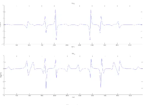
Calculated roll and pitch motions are as presented in Figure 3. The simulated resultant torque training data set is presented in Figure 4.
Figure 3
Smooth roll and pitch motions
The list of non-linear cpFLS parameters consists of six times four integer parameters for defining six fuzzy-partitions having five MFs each, where each partition consists of three classical π-type MFs and for the cpFLS setup one virtual π-type MF composed by one z-type MF at the beginning of the input interval and one s-type MF in the end of the input interval as in equation (8). These six fuzzy- partitions serve as antecedents for the four fuzzy-systems like in equation (9) and (12), used for identifying Dij, ij=(13, 22, 23, 33) as defined in equations (3)-(5) and (14)-(16).
The unknown linear parameter D11 of the multi-rotor model as in equation (15), together with 112 linear parameters of the four TSK FLSs (2 FLSs with 5 MFs on one input, each rule with 2 c parameters, plus 2 FLSs with 5 MFs on both of the 2 inputs, each rule with 3 c parameters) of equations (7) substituted to (9) and (13) are determined by the SVD-based LS method as in equation (17).
Figure 4 Smooth resultant torques
Concluded from equation (8),(10) six fuzzy-partitions (antecedent part of 2 FLSs with 1 input, plus 2 FLSs with 2 inputs are covered by 6 independent fuzzy- partitions) are represented by a vector of six times four parameters, which are optimized by a multi-objective hybrid genetic algorithm as detailed in [14].
Chromosomes are evaluated and subjected to a local gradient based search.
Chromosome values are updated with the result of fine-tuning after each evaluation, so the GA does not waste time on local optimization; only global search capabilities of the GA are utilized.
The GA is set to work on a population of 200 chromosomes, divided into 5 subpopulations, with migration rate 0.2 taking place after each 5 completed generations. Chromosomes are comprised of 24 Gray-coded integers, each consisting of 16 bits. The initial population is set up in a completely random manner. Crossover rate, generation gap and insertion rate is set to 0.8, selection pressure is 1.5. In each generation 4% of individuals are subject to mutation, when 1% of the binary genotype is mutated.
Matrix of the linear equation ℚ(𝒒, 𝒒̇, 𝒒̈) from equation (17) is pre-processed, as FLSs like equation (9) and their partial derivatives like equation (13) are substituted as defined by equations (14)-(16). Unknown linear parameters are D11 and the 112 c parameters of fuzzy-rule consequents.
Evaluation of each individual is conducted as follows:
(a) Convert coded ai values from the chromosome to bk by equation (10).
(b) Evaluate all MFs, and antecedents which will comprise six fuzzy- partitions from each of six bk quadruplets by equations (7) and (8). Also, evaluate antecedent derivatives of equation (13).
(c) Calculated the matrix coefficients of linear equations ℚ(𝒒, 𝒒̇, 𝒒̈) by values of triggered MFs and their partial derivatives.
(d) Linear components [D11, c] of equations (9) and (13) are calculated by SVD decomposition as in (17).
(e) Fine-tune ai parameters, for example by the Matlab “lsqnonlin”
function, while re-calculating steps (a)-(d) for each ai tuning iteration.
(g) Re-insert optimized ai parameters into the evaluated chromosome.
For the multi-objective rank assignment described in [6], the objective vector is created from:
(i) the mean square of the identified torque error, (ii) the maximum absolute torque identification error and (iii) the condition number of the matrix of the linear equation.
Stochastic universal sampling is used for selecting the next generation without explicit elitism. To speed up the GA processing, a database of evaluated chromosomes and their objective vectors is created, so only unique new individuals are evaluated in each generation.
10 Results
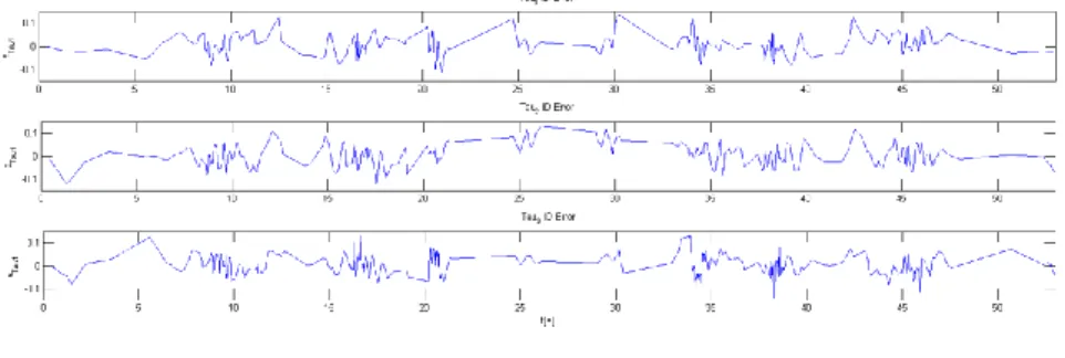
Results of this paper are: (i) a new fuzzy-logic system identification method is defined and validated on an example for a multi-rotor UAV torque dynamic model identification, typical torque identification error is <10%, presented in Figure 7;
(ii) a new bounded, smooth, energy efficient and time optimal trajectory design method is defined and validated on an example for a multi-rotor UAV path planning, a single parameter controls the trajectory dynamics, as presented in Figure 2; (iii) a new training data set reduction algorithm is defined and validated, less than 20% of data points give more than 80% of contribution to the system condition number, a typical rate of condition number change for the most significant 25% of data points is presented in Figure 5.
The basic smooth trajectory parametrization curve used is with P=1, with dt=0.01[s] sampling time, which results in a time optimal trajectory with dynamic boundaries of maximum sinus pop=2𝜋 [m/s6] wave of 1[s] period, maximum crackle=2[m/s5], maximum snap=1[m/s4], maximum jerk=1[m/s3], maximum acceleration=2[m/s2], maximum velocity=8[m/s], displacement=64[m], within
time=16[sec]. The integral of absolute jerk is 8[m/s2], what is proportional to the expended energy (as mass and desired displacement we consider to be constant).
This base trajectory curve is projected to the training path, which results in training data worth of ~55 seconds of flight time.
For uniformly distributed MFs in the fuzzy-partition of antecedents the 𝑐𝑜𝑛𝑑(ℚ𝑓𝑢𝑙𝑙(𝒒, 𝒒̇, 𝒒̈)) condition number (Cond) of the FullTrainingSet and 𝑐𝑜𝑛𝑑(ℚ𝑟𝑒𝑑(𝒒, 𝒒̇, 𝒒̈)) for the ReducedTrainingSet is in Table 4; the condition number change for the first 1170 points out of the total set of 5487 points is presented in Figure 3.
Table 4
Condition number change with changing the size of the reduced trading data set Full set reduced to reduced to reduced to training points
% reduction to 5487 100%
2743 50%
1170 25%
685 12.5%
Cond
% increase by
56254 0%
56805 +0.98%
59771 +6.25%
68934 +22.54%
Figure 5
Condition number changes for the set reduction of 1170 points
Convergence of applied multi objective GAs of population size (Population#) 200, (or 75) is achieved in <200, (or <25) generation evaluations (Generation#), when the typical mean square error (MSE) is <1e-3, the typical maximum torque error (maxE) is <0.2 Nm, which means that the typical relative error is <10%. For fuzzy-partitions defined by non-dominated chromosomes the typical condition number (Cond) of ℚ(𝒒, 𝒒̇, 𝒒̈) the matrix of linear equations is ~4-5000. Averages of 10 simulations for each training data set size are presented in Table 5. For comparison to the new cpFLS model quality results of a simple FLS model, described in [14] are also presented. Results of a selected non dominated model are followed by the average values and the variance of 10 runs of each method and parametrization, as defined in the first 4 rows.
There is neither significant quality, nor identification performance degradation when using the new cpFLS compared to the simple FLS method described in [14].
While the most significant benefit of smooth output transitions for (2kπ-ε) – (0+ε) input space changes of continuous periodic FLSs cannot be achieved by a simple TSK FLS.
In average there is no significant difference in the identification quality for any of the reduced or the full data set. The only real, significant difference is the time required for evaluation, which is proportional to the increased speed of singular value decompositions of different sized samples. The 685 point sample set reduced to 1/8th of the full set is significantly faster evaluated than any other larger set.
Further on the proposed GA setup method is robust enough to compensate for a significant reduction of the GA size parameters as well. The identification result is still very good when reducing the population size to 75 and generations evaluated to 25, which results in a (500*200)/ (75*25)≈5000% fold GA execution time gain.
Table 5
maximum error, means square error and condition number results of identification FLS type FLS[14] cpFLS cpFLS cpFLS cpFLS cpFLS Training points 5487 5487 2743 1170 685 685
Population # 500 500 500 500 500 75
Generation # 200 200 200 200 200 25
MSE selected 0,0007 0,0008 0,0009 0,0009 0,0008 0,0008 maxE selected 0,1531 0,1771 0,1786 0,1648 0,1952 0,2080 Cond selected 2707,1 5506,4 3399,4 4145,9 4262,2 3032,0 MSE mean 0,0008 0,0009 0,0010 0,0010 0,0012 0,0011 MSE variance 0,0001 0,0001 0,0001 0,0002 0,0003 0,0002 maxE mean 0,1845 0,1977 0,2912 0,2329 0,2968 0,2408 maxE variance 0,0324 0,0330 0,2568 0,0540 0,1020 0,0382 Cond mean 3815,5 7342,8 5651,6 6953,7 5368,1 5202,9 Cond variance 1701,2 8493,5 5259,3 5274,6 2434,5 2039,3 Numerical values representing ai of equation (10) for the selected typical non- dominated chromosome are:
[3157 31387 59087 34526 61856 23999 31983 5100 21985 53525 13592 15164 41416 52669 17091 8246 27195 36846 42384 27934 32215 55957 57320 24610], which defines fuzzy-partition MF parameters by equation (10) as:
bi i=1,2,3 for cpFLS modeling D13: [0.024633, 0.26954, 0.7306].
bi i=1,2,3 for cpFLS modeling D22: [0.50315, 0.69836, 0.95851].
bi i=1,2,3 for D23: [0.21085, 0.72421, 0.85457, 0.34681, 0.78784, 0.93095].
bi i=1,2,3 for D33: [0.20241, 0.47664, 0.79209, 0.18939, 0.51835, 0.85532].
The graphical representation of a fuzzy-partition antecedent defined by this chromosome for D33 is shown by Figure 6:
Figure 6
Antecedent fuzzy-partition for D33
The torque identification error along the complete training data set for a cpFLS based quad-rotor model defined by the selected non-dominated chromosome is presented in Figure 7:
Figure 7 Torque identification error
11 Discussion
Simulation results of the proposed new multi-rotor dynamic model identification method by cpFLSs are promising. The quality of identification with the relative torque error being uniformly <10% is suitable for application in model based control algorithms.
The proposed trajectory design method results in real-life feasible smooth, limited torque transients, which is energy efficient for control signal design; while providing a flexible interface to arbitrary velocity, acceleration, jerk and snap limit enforcement. Dynamic transient properties and energy efficiency of the trajectory can be tuned with a single parameter, but the feasibility of torque transients must not be dismissed along this optimization. The resulting trajectory is always the time optimal solution, which complies with all defined limits.
The training data set reduction to 1/8th of the full set significantly increases the identification process speed, while the proposed reduction method ensures that the identification result quality does not deteriorates.
The typical condition number for used linear parameter evaluations is high for the used training data setup, which indicates that the system excitation with this trajectory is insufficient, so a more advanced training trajectory has to be planned with sufficient excitation along the complete input domain.
The new, more advanced training trajectory to be generated should take advantage of the smooth 2π - 0 transition, and it has to be designed so that both roll and pitch input parameters defined by equation are excited along the complete [0, 2π) interval.
References
[1] R. Lozano, “Unmanned Aerial Vehicles,” ISTE Ltd, London, 2010
[2] R. Stengel, “FLIGHT DYNAMICS,” Princeton University Press, Cloth, 2004
[3] C. An, C. Atkeson, J. Hollerbach, “Model-Based Control of a Robot Manipulator,” The MIT Press, Cambridge, 1988
[4] N. Srinivas, K. Deb, “Multiobjective Optimisation Using Nondominated Sorting in Genetic Algorithms,” Evolutionary Computation Vol. 2, No. 3, pp. 221-248, 1994
[5] C. M. Fonseca, P. J. Fleming, “Multiobjective Optimisation and Multiple Constraint Handling with Evolutionary Algorithms I: A Unified Formulation,” University of Sheffield Technical Report No. 564, Sheffield, UK, 1995
[6] A. Nemes, “New Genetic Algorithms for Multi-objective Optimisation,” in proc. of the 1st International Symposium of Hungarian Researchers on Computational Intelligence (HUCI 2000), Budapest, 2000
[7] G. Carrillo, D. López, R. Lozano, C. Pégard, “Modeling the Multi-rotor Mini-Rotorcraft,” Quad Rotorcraft Control, Springer, 2013
[8] M. Spong, M. Vidyasagar, “Robot Dynamics and Control,” John Wiley and Sons, Inc. 1989
[9] L. Wang, “Adaptive Fuzzy Systems and Control, Design and Stability Analysis,” PTR Prentice Hall, 1994
[10] H. Hellendron, D. Driankov, “Fuzzy Model Identification, Selected approaches,” Springer, 1997
[11] A. Nemes, “Function Identification by Unconstrained Tuning of Zadeh- type Fuzzy Partitions,” in proc. of the 2nd International Symposium of
Hungarian Researchers on Computational Intelligence (HUCI 2001), Budapest, 2001
[12] J. Jang, C. Sun, E. Mizutani, “Neuro-Fuzzy and Soft Computing, A Computational Approach to learning and Machine Intelligence,” Prentice- Hall, 1997
[13] A. Nemes, B. Lantos “Training Data Reduction for Optimisation of Fuzzy Logic Systems for Dynamic Modeling of Robot Manipulators by Genetic Algorithms,” in proc. of the IEEE Instrumentation and Measurement Technology Conference (IMTC 2001), Vol. 3, pp. 1418-1423, 2001
[14] A. Nemes, “Genetic Fuzzy Identification Method for Qadrotor UAVs,”
ANNALS of Faculty Engineering Hunedora, Vol. 13, No. 3, 2015
[15] A. Rodic, G. Mester, “Sensor-based Navigation and Integrated Control of Ambient Intelligent Wheeled Robots with Tire-Ground Interaction Uncertainties,” Acta Polytechnica Hungarica, Vol. 10, No. 3, pp. 113-133, 2013
[16] A. Rodic, G. Mester, “Virtual WRSN – Modeling and Simulation of Wireless Robot-Sensor Networked Systems,” in proc. of the 8th IEEE International Symposium on Intelligent Systems and Informatics (SISY 2010), pp. 115-120, 2010
[17] G. Mester, “Introduction to Control of Mobile Robots,” in proc. of the YUINFO 2006, pp. 1-4, 2006
[18] G. Mester, “Improving the Mobile Robot Control in Unknown Environments,” in proc. of the YUINFO 2007, pp. 1-5, 2007
[19] G. Mester, “Adaptive Force and Position Control of Rigid Link Flexible- Joint SCARA Robots,” in proc. of the 20th IEEE International Conference on Industrial Electronics, Control and Instrumentation (IECON'94), Vol. 3, pp. 1639-1644, 1994