Sobolev gradient preconditioning for elliptic reaction–

Sobolev gradient preconditioning for elliptic reaction–

diffusion problems with some nonsmooth nonlinearities

J. Kar´atson¹ Abstract

The Sobolev gradient approach is an efficient way to construct preconditioned iterations for solving nonlinear problems. We extend this technique to be applicable for elliptic equations describing stationary states of reaction–diffusion problems if the nonlinearities have certain lack of differentiability. We derive convergence results of the Sobolev gradient method on an abstract level and then for our elliptic problem under different assumptions. Numerical tests show convergence as expected.

Keywords. Sobolev gradients, iteration, nonlinear elliptic equation

1 Introduction

Reaction–diffusion problems arise in various nonlinear models in applied mathematics, see, e.g., [7, 14] and the references there. It is often of interest to determine station- ary states, which are described by elliptic problems. In order to solve numerically the arising nonlinear problems, an efficient approach is the Sobolev gradient method. The foundations and various contexts of the Sobolev gradient method have been described in [15, 16], for problems with potential see also the author’s works [4, 9]. The main idea is that the gradient w.r.t. the Sobolev inner product provides a properly precon- ditioned iteration. Sobolev gradients have been succesfully used in many applications in the recent decade, such as image processing, Burgers’ and Navier-Stokes equations, differential-algebraic equations, Gross-Pitaevskii equations and Ginzburg-Landau func- tionals, see [11, 12, 17, 18, 19, 20, 21]. Compared to Newton-like methods, which require less iterations, the Sobolev gradient approach often proves to be be still more favourable due to the simpler linearized problems (that, moreover, do not vary in course of the it- eration process) and since it is directly fitted to minimization settings. A systematic comparison on a model problem has been executed in [13].

The standard convergence results for such iterations rely on suitable smoothness of the nonlinearity that describes the chemical reaction in the elliptic equation. In this paper we study problems where this smoothness condition is relaxed, and hence the above results cannot be applied. In general, we consider semilinear elliptic boundary value problems of the following form:

−div k∇u

+q(x, u) = g,

u|∂Ω = 0, (1.1)

with a diffusion coefficient k ∈L^∞(Ω), k ≥m > 0, and with a continuous nonlinearity q such that ξ 7→q(x, ξ) is increasing for any x ∈Ω. Later we will impose further technical restrictions on q to have well-posedness and then to achieve more concrete estimates on

1Department of Applied Analysis & MTA-ELTE Numerical Analysis and Large Networks Research Group, ELTE University; Department of Analysis, Technical University; Budapest, Hungary

the order of convergence of Sobolev gradients. However, these assumptions will still allow nonsmoothness of q. A typical example of such a nonlinearity is q(x, u)≡ q(u) = u^γ for u > 0 (or rewritten as |u|^γ−1u for any u) with some exponent 0 < γ < 1, see, e.g., [3].

Further details on this example will be mentioned later.

Note that for such nonlinear problems it is not possible to apply Newton’s method.

Moreover, semismooth Newton methods are not applicable either for such non-Lipschitz functions, since semismoothness requires at least local Lipschitz continuity [8] and is thus typically used for nonlinearities like e.g. max{u,0}.

As mentioned above, the Sobolev gradient method provides a properly preconditioned iteration by taking gradients w.r.t. the Sobolev inner product. An elegant property of this approach is that both the construction and the study of convergence can be carried out in the Sobolev space associated to the PDE, that is, on the continuous level. Then one can readily derive the analogous results for finite element discretizations using a proper projection into the FEM subspace, moreover, convergence is typically mesh-independent, see [4, 9]. We follow this vein in this paper, and we focus on the continuous level in the Sobolev space H₀¹(Ω). After a proper foundation of the problem and of underlying Hilbert space techniques, we derive convergence results of the Sobolev gradient method for our elliptic problem under different assumptions. Thus we obtain generalizations of the existing Sobolev gradient results.

2 The problem and its well-posedness

Let Ω⊂R^d be a bounded domain, and let problem (1.1) satisfy the following Assumptions 2.1.

(i) k ∈L^∞(Ω), k ≥m >0;

(ii) q: Ω×R→R is continuous;

(iii) ξ 7→ q(x, ξ) is increasing for any x ∈ Ω, further, there exists a number p ≥ 1 (if d= 2) or 1≤p≤ _d−2^2d (if d >2) such that

|q(x, ξ)| ≤c1+c2|ξ|^p−1 (∀x∈Ω, ξ ∈R); (2.1) (iv) g ∈L²(Ω).

The bound for the exponent p in (2.1) ensures the following Sobolev embedding, which will be required for the well-posedness:

H₀¹(Ω)⊂L^p(Ω), kvk_L^p ≤C_pkvk_H¹

0 (∀v ∈H₀¹(Ω)) (2.2) for some constant C_p > 0 independent of v, see [1, Theorem 5.4]. The weak form of the problem reads in a usual way as follows: find u∈H₀¹(Ω) such that

Z

Ω

k∇u· ∇v+q(x, u)v

= Z

Ω

gv (∀v ∈H₀¹(Ω)). (2.3)

Proposition 2.1 Problem (1.1) has a unique weak solution.

Proof. Let us consider the Hilbert space H₀¹(Ω) with inner product hu, vi_H¹

0 :=

Z

Ω

∇u· ∇v, (2.4)

and the functional φ:H₀¹(Ω)→R, φ(u) :=

Z

Ω

k

2|∇u|²+Q(x, u)−gu ,

where Q is a potential of q w.r.t. ξ, i.e. Q : Ω×R → R satisfies ∂_ξQ(x, ξ) = q(x, ξ) for allx, ξ. The estimate (2.1) implies a bound|Q(x, u)| ≤c˜₁+ ˜c₂|u|^p, hence the embedding H₀¹(Ω)⊂L^p(Ω) ensures that the integral in φ(u) is finite. Using standard techniques, one can check the Gateaux differentiability ofφ: namely, for any u, v ∈H₀¹(Ω), there exists hφ⁰(u), vi_H¹

0 = lim

t→0

1

t φ(u+tv)−φ(u)

= Z

Ω

k∇u·∇v−gv +limt→0

Z

Ω

t^k₂|∇v|²+∂_ξQ(x, u+tθv)v

= Z

Ω

k∇u· ∇v+q(x, u)v −gv

, (2.5)

where the last step follows because the integrand converges a.e. ast→0 and is majorized owing to (2.1). The functional φ has the following properties. It is uniformly convex, since Q is convex by the monotonicity of q. Further, the convexity of Q also implies Q(x, ξ)≥Q(x,0) +∂_ξQ(x,0)ξ=q(x,0)ξ if we choose Q such thatQ(x,0)≡0. Hence

φ(u)≥ Z

Ω

k

2 |∇u|²+q(x,0)u−gu

≥ ^m₂kuk²_H1

0 −(kq(x,0)k_L² +kgk_L²)kuk_L²

≥ ^m₂kuk²_H1

0 −ckuk_H¹

0 → +∞ as kuk_H¹

0 →+∞.

As is well-known (see, e.g., [25, Theorem 40.1]), these properties imply thatφhas a unique minimizer, which is also its unique critical point, that is, where hφ⁰(u), vi_H¹

0 = 0 for all v ∈H₀¹(Ω). In virtue of (2.3) and (2.5), this minimizer is the unique weak solution of our problem.

Example. A typical example for a reaction-diffusion problem with nonsmooth non- linearity is

−∆u+u^γ = g,

u|∂Ω = 0, (2.6)

where 0< γ <1 is the order of the reaction, see, e.g., [3]. The increasing functionu7→u^γ describes an autocatalytic (endothermic) reaction, defined foru≥0. One can extend this function in an increasing manner asu7→ |u|^γ−1u for any u∈R, and for source functions g ≥0 the maximum–minimum principle ensures that the solution of the problem

−∆u+|u|^γ−1u = g,

u|∂Ω = 0 (2.7)

is nonnegative, hence the solutions of (2.6) and (2.7) coincide. In this example the non- smoothness of q comes from non-differentiability in one point only (u = 0), but even this fact prohibits the applicability of some standard solution techniques. Note that the above nonlinearity is H¨older continuous, which will be a main assumption later to achieve more concrete estimates on convergence. Although this will be a strengthened continuity assumption, it is still general. It allows non-differentiability of q at even infinitely many points, as is the case with Cantor’s function (or devil’s staircase).

The weak form of our problem can be rewritten as an operator equation as follows.

The Riesz repesentation theorem provides an operatorF :H₀¹(Ω)→H₀¹(Ω) for which hF(u), vi_H¹

0 =

Z

Ω

k∇u· ∇v+q(x, u)v −gv

(∀v ∈H₀¹(Ω)). (2.8) Thus (2.3) becomes

hF(u), vi_H¹

0 = 0 (∀v ∈H₀¹(Ω)), or simply

F(u) = 0. (2.9)

We wish to solve (2.9) with a steepest descent (or gradient) type method, based on the underlying potential φ. For this purpose, we first formulate general results in a Hilbert space setting.

3 Some results on steepest descent iterations in Hilbert space

LetH be a real Hilbert space andF :H →H be a potential operator, i.e. there exists a Gateaux differentiable functional φ:H →R such that

φ⁰ =F.

Further, assume that F is uniformly monotone, i.e. there exists m >0 such that

hF(v)−F(u), v−ui ≥mkv−uk² (∀u, v ∈H). (3.1) We wish to solve the equation

F(u) = 0.

The uniformly monotonicity assumption implies that there is a unique solution u^∗ ∈ H, which coincides with the minimizer of φ, see, e.g., [25]. Further, it is not restrictive to have a zero r.h.s., since any equation F(u) = b can be rewritten as F(u)−b = 0 with an operator u7→F(u)−b satisfying the same conditions as F.

The steepest descent iteration is a sequence of fixed-point iteration form:

u_n+1 :=u_n−α_nF(u_n) (3.2)

with suitable constants α_n > 0. In this case the search direction is −F(u_n) = −φ⁰(u_n).

We present some convergence results under various continuity conditions on F.

We start with a general theorem, where we assume that F is uniformly continuous in the following sense: there exists a real function r :R⁺ →R⁺ such that

r is continuous and increasing; (3.3)

r(0) = 0, lim

t→+∞r(t) = +∞; (3.4)

kF(u)−F(v)k ≤ r(ku−vk) (∀u, v ∈H). (3.5) On the other hand, typically the functionr has some simpler special form, such asr(t) = Lt for Lipschitz continuity or r(t) = Lt^α for H¨older continuity. Hence we will later formulate the rate of convergence for these situations.

The following discussion will use the integral and average functions of r, respectively:

R(t) :=

Z t

0

r(s)ds , ρ(t) := 1 t

Z t

0

r(s)ds = R(t)

t . (3.6)

Theorem 3.1 Let F satisfy conditions (3.1) and (3.3)–(3.5). Then, for stepsizes α_n := _kF(u¹

n)k ρ^{−1 kF(u}₂^n)k

, (3.7)

the error of iteration (3.2) satisfies

e_n :=ku_n−u^∗k →0.

Proof. The Newton-Leibniz formula yields φ(u_n+1)−φ(u_n) =

Z 1

0

hF u_n+t(u_n+1−u_n)

, u_n+1−u_nidt .

Subtracting hF(u_n), u_n+1−u_ni, using (3.5) and (3.6), we obtain φ(u_n+1)−φ(u_n)− hF(u_n), u_n+1−u_ni ≤

Z 1

0

r tku_n+1−u_nk

ku_n+1−u_nkdt

=

Z kun+1−unk

0

r(s)ds = R ku_n+1−u_nk . Using (3.2), we have

φ(u_n+1)−φ(u_n)≤ −α_nkF(u_n)k²+R α_nkF(u_n)k .

Now let us define α_n as in (3.7). This makes sense since (owing to the assumptions)ρ is increasing and lim+∞ρ= +∞. Then

R α_nkF(u_n)k

=α_nkF(u_n)kρ α_nkF(u_n)k

=α_n^kF(un)k

2

2 ,

hence

φ(u_n+1)−φ(u_n)≤ −α_n^kF(u₂^n)k2 = −^kF(u₂^n)kρ^{−1 kF(u}₂^n)k

=: −σ(kF(u_n)k), where

σ(t) := ₂^t ρ⁻¹ ₂^t

is increasing and σ(0) = 0.

Thus ∞

X

n=0

σ(kF(u_n)k)≤

∞

X

n=0

φ(u_n) −φ(u_n+1)

=φ(u₀)−infφ =:D < ∞, (3.8) hence σ(kF(un)k)→0 and thuskF(un)k →0 as n → ∞. Finally, from (3.1),

mku_n−u^∗k ≤ kF(u_n)−F(u^∗)k=kF(u_n)k →0 (3.9) i.e. the theorem is proved.

Estimates on the rate of convergence can be given under special choices on r. In each case it suffices to estimate kF(u_n)k, since one can use (3.9). First we consider H¨older continuity.

Theorem 3.2 Let F be H¨older continuous, i.e. satisfy condition (3.5) with r(t) :=M t^γ for some constants M >0 and 0< γ≤1, and also satisfy (3.1). Then, with stepsizes α_n from (3.7), for some constant c1 >0,

0≤k≤nmin e_k ≤c₁n⁻

γ

γ+1 (∀n∈N). (3.10)

Proof. We follow [24], where the situation of H¨older continuity was considered for optimization on a finite dimensional space. For the function r(t) := M t^γ, one can see that σ(t) =c₀t^γ+1γ with some c₀ >0. Here

c0 min

0≤k≤nkF(uk)k^γ+1γ = min

0≤k≤nσ(kF(uk)k)≤ _n¹

n

X

k=0

σ(kF(uk)k)≤ ^D_n with D from (3.8), hence (3.9) yields

0≤k≤nmin e_k≤ _m¹ min

0≤k≤nkF(u_k)k ≤c₁n⁻

γ γ+1 .

Remark 3.1 (i) The stepsize for r(t) := M t^γ can be obtained with an elementary calcu- lation from (3.7) :

α_n = ^γ+1_2M

1

γkF(u_n)k^γ1−1. (3.11)

(ii) For Theorem 3.2 to hold, it suffices to require H¨older continuity of r in a proper neighbourhood of 0, since the proof use this property for arguments that tend to 0. In other words, it suffices to require local H¨older continuity ofF: for any R >0 there exists a constantM > 0 such that

kF(u)−F(v)k ≤Mku−vk^γ (∀u, v ∈H₀¹(Ω) whenever kuk, kvk ≤R). (3.12)

In the case of Lipschitz continuity the above proof (forγ = 1) would yield convergence ofO(n⁻¹²). However, with some further regularity properties, we then have even geometric (i.e., linear) convergence:

Theorem 3.3 Let F be Lipschitz continuous, i.e. satisfy condition (3.5) withr(t) :=M t for some constant M > 0, and also satisfy (3.1). Assume also that F itself is Gateaux differentiable, the operators F⁰(u) are self-adjoint, and F⁰ is hemicontinuous (i.e. weakly continuous on segments). Then, using constant stepsizes α := _M+m² , denoting c₁ :=

1

mkF(u₀)k, we have

e_n≤c₁

M −m M +m

ⁿ

(∀n∈N).

Proof. Under the assumptions onF⁰, the uniform monotonicity and Lipschitz continuity conditions are equivalent to requiring

mkhk² ≤ hF⁰(u)h, hi ≤Mkhk² (∀u, h∈H), in which situation the result is well-known, see, e.g., [4, Theorem 5.4].

4 Sobolev gradients on continuous and discrete level

Now we study the numerical solution of the boundary value problem (1.1), based on the results of the previous section. As described in the introduction, one may first for- mulate the iteration on the Sobolev space level. Then the iteration for a finite element discretization is obtained just by a projection into the FEM subspace used.

4.1 Sobolev gradient preconditioning

In our case, where F = φ⁰, the gradients of φ are used to solve equation F(u) = 0.

The Sobolev gradient iteration is defined by taking gradients w.r.t. the Sobolev inner product. This leads to linearized problems in each step, i.e. a properly preconditioned iteration. The linearized problems depend on the inner product used; we consider two situations. The standardH₀¹(Ω) inner product leads to auxiliary Poisson equations, which is favourable if there is an efficient Poisson solver to be used. If a weighted inner product is applied in H₀¹(Ω), then one can simplify the iteration.

Sobolev gradients with the standard H₀¹(Ω) inner product. Letu0 ∈H₀¹(Ω) be an arbitrary initial guess. For givenu_n (n∈N), the iteration step (3.2) can be written as

z_n:=F(u_n), u_n+1 :=u_n−α_nz_n, where

α_n:= ^γ+1_2M

1

γkF(u_n)k

1 γ−1

H₀¹ or α_n ≡α := _M+m² (4.1) when the conditions of Theorem 3.2 or Theorem 3.3 hold, respectively. Herez_n :=F(u_n) is equivalent to

hz_n, vi_H¹

0 =hF(u_n), vi_H¹

0 (∀v ∈H₀¹(Ω)), (4.2)

i.e. z_n ∈H₀¹(Ω) is the function that satisfies Z

Ω

∇zn· ∇v = Z

Ω

k∇un· ∇v+q(x, un)v −gv

(∀v ∈H₀¹(Ω)). (4.3) That is, altogether, the iteration has the following form:

u_n+1 :=u_n−α_nz_n, (4.4)

where z_n is the weak solution of the linear elliptic problem −∆z_n = −div k∇u_n

+q(x, u_n)−g,

z_n|∂Ω = 0. (4.5)

Weighted Sobolev gradients. Now let us use the weighted inner product

hu, vi_H¹

0 :=

Z

Ω

k∇u· ∇v (4.6)

adapted to the problem. Then, instead of (4.5), z_n is the weak solution of the linear elliptic problem

−div k∇z_n

= −div k∇u_n

+q(x, u_n)−g,

z_n|∂Ω = 0. (4.7)

In this case the iteration can be rewritten in the following simpler form: letting w_n:=z_n−u_n,

if wn is the weak solution of the linear elliptic problem −div k∇w_n

= q(x, u_n)−g,

z_n|∂Ω = 0. (4.8)

then

un+1 := (1−αn)un−αnwn. (4.9) Here α_n is from (4.1), understanding the H₀¹(Ω)-norm with weight function k added in (2.4).

4.2 Finite element discretization

The finite element method (FEM) looks for the numerical solution of problem (2.3) in a proper FEM subspace Vh ⊂H₀¹(Ω): find u∈Vh such that

Z

Ω

k∇u· ∇v+q(x, u)v

= Z

Ω

gv (∀v ∈V_h). (4.10)

The Sobolev gradient iteration for the FEM problem (4.10) is directly obtained with the projection of (4.3) into V_h. Namely, let u₀ ∈ V_h be an arbitrary initial guess. For given un (n ∈N), we let un+1 :=un−αnzn, wherezn ∈Vh is the function that satisfies

Z

Ω

∇zn· ∇v = Z

Ω

k∇un· ∇v +q(x, un)v −gv

(∀v ∈Vh), (4.11) i.e. z_n ∈V_h is the FEM solution of the linear elliptic problem (4.5), if the standard inner product is used. Finally, for weighted Sobolev gradients, we have the weight function k on the l.h.s. of (4.11), and the iteration can be simplified with wn in the obvious way.

We note that the estimates are independent of the actual FEM subspace used. This property will also be reflected in the mesh independence obtained in the numerical tests in subsection (5.3).

5 Convergence estimates

5.1 Power order convergence

In this subsection we establish convergence rates under the assumption of H¨older conti- nuity ofq, i.e., we impose

Assumption 5.1. The function q is H¨older continuous w.r.t. ξ, i.e., there exist constants c_q >0 and 0< γ < 1 such that

|q(x, ξ)−q(x,ξ)| ≤˜ cq|ξ−ξ|˜^γ (∀x∈Ω, ξ ∈R). (5.1)

Proposition 5.1 The operator F in (2.8) is locally H¨older continuous on H₀¹(Ω) in the sense of (3.12).

Proof. The operator F can be decomposed in a linear and a remaining part as F =L+A,

where

hLu, vi_H¹

0 =

Z

Ω

k∇u· ∇v, hA(u), vi_H¹

0 =

Z

Ω

q(x, u)v −gv

(∀v ∈H₀¹(Ω)).

First, Lis Lipschitz continuous since it is a bounded linear operator:

kLuk_H¹

0 = sup

kzk_H1 0

=1

hLu, zi_H¹

0 = sup

kzk_H1 0

=1

Z

Ω

k∇u· ∇z ≤ kkk_L^∞k∇uk_L² =kkk_L^∞kuk_H¹

0,

hence it is locally H¨older continuous. Second, we prove thatAis H¨older continuous. Here kA(u)−A(v)k_H¹

0 = sup

kzk_H1 0

=1

hA(u)−A(v), zi_H¹

0 = sup

kzk_H1 0

=1

Z

Ω

q(x, u)−q(x, v) z

≤c_q sup

kzk_H1 0

=1

Z

Ω

|u−v|^γ|z|.

We can first apply H¨older’s inequality with the parameters ^γ+1_γ and γ+ 1, since _γ+1^γ +

1

γ+1 = 1, and then the Sobolev embedding

kwk_L^γ+1 ≤C_γ+1kwk_H¹

0 (5.2)

from (2.2), since γ+ 1 ≤2≤ _d−2^2d . Thus we obtain Z

Ω

|u−v|^γ|z| ≤

|u−v|^γ

L

γ+1

γ kzk_Lγ+1 =ku−vk^γ_Lγ+1kzk_Lγ+1 ≤C_γ+1^γ+1ku−vk^γ_H1 0

kzk_H¹

0 . The above inequalities yield

kA(u)−A(v)k_H¹

0 ≤c_qC_γ+1^γ+1ku−vk^γ_H1

0 (5.3)

that is, A is H¨older continuous (globally, and hence locally). Altogether, F = L+A is also locally H¨older continuous.

Theorem 5.1 Let Assumptions 2.1 and 5.1 hold. Let us construct the Sobolev gradient iteration, starting from arbitrary initial guess u₀ ∈H₀¹(Ω), according to either (4.4)–(4.5) or (4.8)–(4.9), and choose the stepsizes αn from (3.11). Then, for some constant c1 >0, the errors e_k :=ku_k−u^∗k_H¹

0 satisfy

0≤k≤nmin e_k ≤c₁n⁻

γ γ+1 .

Proof. Proposition 5.1 and Remark 3.1 yield that Theorem 3.2 can be applied for F inH₀¹(Ω) with inner product (2.4), hence the corresponding Sobolev gradient iteration (4.4)–(4.5) satisfies (3.10). Further, the weighted inner product (4.6) induces a norm equivalent to the original one, hence Proposition 5.1 also holds w.r.t. the weighted norm, and hence the weighted Sobolev gradient iteration (4.8)–(4.9) also satisfies (3.10).

Remark 5.1 In order to calculate the stepsize (3.11), we need the values γ, kF(u_n)k_H¹

0

and M.

• Hereγ is known since it coincides with the H¨older constant ofq from (5.1).

• By construction, F(un) =: zn is computed as the solution of the auxiliary linear problem, hence we have to computekz_nk_H¹

0 after solving the auxiliary problem and use this value in the stepsize.

• For M we can use any bound with which the H¨older continuity estimate holds.

As seen in the proof of Proposition 5.1, such a bound requires an estimate for the

embedding constant C_γ+1 that appears in (5.3). For a simple estimate for this, we can use the intermediate L² space, since, as is well-known, for anyβ ≤2

kwk_L^β ≤ |Ω|^β1−12kwk_L², kwk_L² ≤ ^diam(Ω)_d^√_π kwk_H¹

0, see [4, 22]. Hence, with β =γ+ 1, we obtain that (5.2) holds with

C_γ+1 ≤ _2(1+γ)^{1−γ diam(Ω)}_d^√_π .

5.2 Local linear convergence for interior regular problems

In this subsection we study a special subclass of our boundary value problem (1.1). The main assumption is that the nonsmoothness of the nonlinearity (i.e. the singularity of its derivative) is restricted to the argument ξ= 0, as formulated below (5.5). As it will turn out, positive source functions implyu >0 inside Ω, hence the singularity of such problems is restricted to the boundary where u= 0. This situation still covers the example (2.6).

Let us consider the problem

−∆u+q(x, u) = g,

u|∂Ω = 0 (5.4)

under the following Assumptions 5.2.

(i) Ω⊂R² is a bounded domain, and ∂Ω∈C¹;

(ii) q: Ω×R→R is continuous, further, q(x,0) = 0 (∀x∈Ω);

(iii) for anyx∈Ω, ξ7→q(x, ξ) is increasing and it isC¹ onR\ {0}, further, there exist constants 0< γ < 1 and cγ >0 such that

|∂ξq(x, ξ)| ≤cγ|ξ|^γ−1 (∀x∈Ω, ξ ∈R\ {0}); (5.5) (iv) g ∈C(Ω) and g >0 in Ω.

Remark 5.2 Assumptions 5.2 clearly imply that Assumptions 2.1 and 5.1 hold, i.e. we have a subclass of the previous boundary value problem. Namely, the diffusion coefficient is now k ≡ 1, further, using the Newton–Leibniz-formula, (5.5) implies both the H¨older continuity and the growth condition for q.

5.2.1 Properties of the exact solution

The positivity features of the solution will play an important role. For this we fomulate the following property, where ∂_νu denotes the outer normal derivative.

Definition 5.1 A function u : Ω →R is called strongly positive on Ω if u ∈C¹(Ω) and it satisfies u >0 on Ω and ∂_νu <0 on ∂Ω.

Lemma 5.1 If u is strongly positive, then |u|^γ−1 ∈L^r(Ω) for any 1< r < _1−γ¹ .

Proof. Since ∂_νu <0 is continuous on ∂Ω, there exists m > 0 such that∂_νu ≤ −m on∂Ω. For given x∈Ω, let d(x) denote the distance of xfrom∂Ω, and letx₀ ∈∂Ω such that d(x) = |x−x₀|. For given δ >0, let Ω_δ :={x ∈ Ω : d(x) < δ}. Then there exists δ >0 such that u(x)≥ ^m₂|x−x₀| forx∈Ω_δ. Hence

|u(x)|^r(γ−1) ≤c|x−x₀|^r(γ−1) (∀x∈Ω_δ),

and since r(γ −1) > −1, we have |u|^r(γ−1) ∈ L¹(Ω_δ), i.e. |u|^γ−1 ∈ L^r(Ω_δ). Further, u≥ε:= minΩ\Ω_δ >0 in Ω\Ω_δ, thus |u|^γ−1 ∈L^r(Ω\Ω_δ). Altogether, |u|^γ−1 ∈L^r(Ω).

Proposition 5.2 The solution of (5.4) is strongly positive.

Proof. It follows from [6, Theorem 12.4] that u ∈C¹(Ω). Now, first we prove that u >0. Under our monotonicity and positivity assumptions, we haveu≥0 (see, e.g., [10]), hence we only have to exclude interior zeros. Assume for contrary that there existsx₁ ∈Ω such that u(x₁) = 0. Then x₁ is a local minimizer, hence ∆u(x₁) ≥ 0. Further, from assumption (ii),u(x₁) = 0 implies q(x₁, u(x₁)) = 0, and from assumption (iv), g(x₁)>0.

These lead to the contradiction

0≥ −∆u(x₁) + q(x₁, u(x₁)) =g(x₁)>0.

Now we prove∂_νu <0 on∂Ω. By the strong maximum principle [6, Lemma 3.4], we have

∂νu(x0)< 0 for x0 ∈∂Ω whenever u(x0)< u(x) for all x∈ Ω. In our case this holds on the whole ∂Ω, since u(x₀) = 0 and u >0 in Ω.

Corollary 5.1 For any 1 < r < _1−γ¹ , the solution of (5.4) satisfies |u|^γ−1 ∈ L^r(Ω). In other words,

I_r(u) :=

Z

Ω

|u|^r(γ−1) < ∞. (5.6)

5.2.2 The local linear convergence result

Based on the above, we are able to provide linear rate of convergence (hence an accelera- tion if compared with the bound in Theorem 5.1) provided thatu_n is close enough to the exact solution to reproduce its positivity properties, formulated in Proposition 5.2 and Corollary 5.1. Namely, let us impose

Assumptions 5.3. There exists n₀ ∈N such that (i) un is strongly positive for any n≥n0;

(ii) K_r := sup

n≥n₀

I_{r|[un, un+1]} < ∞.

Here we used notation sup

n≥n0

I_r|[un, un+1] := sup

n≥n0

{I_r(u) : u=su_n+ (1−s)u_n+1, 0≤s≤1}.

Lemma 5.2 If (5.6) holds, then the Gateaux derivative of F satisfies mkhk²_H1

0 ≤ hF⁰(u)h, hi_H¹

0 ≤

˜

m+c_γC_2s² I_r(u)^1r khk²_H1

0 (∀h∈H₀¹(Ω)).

Proof. It follows in a standard way [4] that the Gateaux derivative of F satisfies hF⁰(u)h, vi_H¹

0 =

Z

Ω

k∇h· ∇v+∂_ξq(x, u)hv

(∀h, v ∈H₀¹(Ω)).

To prove the upper bound, let us fix some number 1 < r < _1−γ¹ . We can use H¨older’s inequality with the parameters r and s:= _r−1^r , since ¹_r + ^r−1_r = 1. Then, with (2.2),

Z

Ω

|u|^γ−1h² ≤

|u|^γ−1 L^r

h²

L^s =I_r(u)^1r khk²_L2s ≤I_r(u)^1r C_2s² khk²_H1 0 , hence, letting ˜m := sup_Ωk,

hF⁰(u)h, hi_H¹

0 =

Z

Ω

k|∇h|²+∂_ξq(x, u)h²

≤m˜ Z

Ω

|∇h|²+c_γ Z

Ω

|u|^γ−1h²

≤

˜

m+c_γC_2s² I_r(u)^1r khk²_H1

0 . The lower bound follows readily: since ∂_ξq≥0, we have

mkhk²_H1

0 =m

Z

Ω

|∇h|² ≤ Z

Ω

k|∇h|² ≤ hF⁰(u)h, hi_H¹

0 .

Now we are in the position to prove linear convergence, for which we can adapt the techniques of [4, Theorem 5.4] in order to derive a local version of Theorem 3.3.

Theorem 5.2 Let Assumptions 5.2–5.3 hold. Let us construct the Sobolev gradient iter- ation as in Theorem 5.1, but for n ≥ n₀ redefine the stepsize as a constant α_n ≡ α :=

2

M+m, where M := ˜m + c_γC_2s² Kr^1/r. Then, denoting c₁ := _m¹kF(u_n0)k_H¹

0, the errors en :=kun−u^∗k_H¹

0 satisfy

en≤c1

M −m M+m

ⁿ⁻ⁿ⁰

(∀n≥n0).

Proof. In virtue of the Newton-Leibniz formula, and sinceun+1 :=un−α F(un), F(u_n+1) = F(u_n) +

Z 1

0

F⁰ u_n+t(u_n+1−u_n)

(u_n+1−u_n)dt

=F(u_n)−α Z 1

0

F⁰ u_n+t(u_n+1−u_n)

F(u_n)dt =:L_nF(u_n), where

L_n:=I−α Z 1

0

F⁰ u_n+t(u_n+1−u_n) dt

is a bounded linear operator on H₀¹(Ω), which is self-adjoint since the derivatives F⁰(u) of the potential operator F are self-adjoint. Moreover, for any u :=u_n+t(u_n+1−u_n)∈ [un, un+1] and h∈H₀¹(Ω), Lemma 5.2 and Assumption 5.3 (ii) yield

mkhk²_H1

0 ≤ hF⁰(u)h, hi_H¹

0 ≤Mkhk²_H1

0 , where M := ˜m+c_γC_2s² K

1

rr, hence

(1−αM)khk²_H1

0 ≤ hL_nh, hi_H¹

0 ≤(1−αm)khk²_H1 0 .

The stepsize α = _M²_+m yields 1 −αm = −(1−αM) = ^M_M^−m_+m, hence kLnk ≤ ^M_M^−m_+m. Thus

kF(u_n+1)k_H¹

0 ≤ ^M_M^−m_+mkF(u_n)k_H¹

0 (∀n ≥n₀).

This and (3.9) altogether yield e_n ≤ _m¹kF(u_n)k_H¹

0 ≤ _m¹kF(u_n0)k_H¹

0

_M−m

M+m

n−n0

(∀n≥n₀).

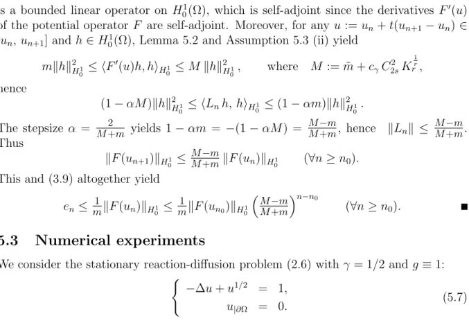
5.3 Numerical experiments

We consider the stationary reaction-diffusion problem (2.6) with γ = 1/2 and g ≡1:

( −∆u+u^1/2 = 1,

u|∂Ω = 0. (5.7)

For instance, such an equation with exponent 1/2 can describe the concentration u of chlorine in a gas phase reaction with chloroform if the latter has a larger magnitude considered as constant [23].

We used Courant finite elements on the unit square domain. For this problem, owing to the Laplacian principal part, the standard and weighted Sobolev gradients (4.5) and (4.7) coincide. We have run the iteration with three mesh parameters h, and calculated the residual errors and convergence quotients

ε_n :=kF(u_n)k_H¹

0 and Q_n:= ε_n

εn−1

,

respectively. Owing to the positivity of the iterates, we have used the simple formu^1/2 of the nonlinearity in the code instead of |u|^−1/2u. The results are shown in Table 1.

h= 0.1 h= 0.01 h= 0.001

ε_n Q_n ε_n Q_n ε_n Q_n

0.1814322 0.1874409 0.1874726

0.0301495 0.1661 0.0302984 0.1617 0.0302977 0.1616 0.0019173 0.0636 0.0018617 0.0614 0.0018612 0.0614 0.0001317 0.0687 0.0001235 0.0663 0.0001234 0.0663 0.0000089 0.0683 0.0000081 0.0660 0.0000081 0.0659 0.0000006 0.0684 0.0000005 0.0661 0.0000005 0.0660

Table 1. The residual errors and convergence quotients for the test problem.

One may observe that the convergence is linear in accordance with subsection 5.2, further, it shows a uniform behaviour independently of the mesh size h.

5.4 Concluding remarks

We have established the rate of convergence of the Sobolev gradient iteration in two situations in the Sobolev space H₀¹(Ω). For the finite element discretization, the iteration is obtained just by a projection into the FEM subspace. The convergence estimates for the FEM case coincide with the Sobolev space case, since the proofs that use functions in H₀¹(Ω) can be restricted to functions inV_h only. This approach is similar to the one used in [4, 15].

Besides obtaining convergence of Sobolev gradients, we mention that Newton’s method or its semismooth versions might not be used here owing to the lack of Lipschitz continuity.

Finally we note that our results can be generalized in a straightforward way to certain more general situations: to problems with mixed boundary conditions and for gradient systems, i.e. PDE systems arising from the minimization of a joint energy functional. In these cases the Sobolev spaceH₀¹(Ω) has to be replaced by a subspace ofH¹(Ω) associated to the given Dirichlet portion of the boundary, or by a product Sobolev space, respectively.

Acknowledgements. This research was carried out in the ELTE Institutional Excellence Program (1783-3/2018/FEKUTSRAT) supported by the Hungarian Ministry of Human Capacities, and supported by the Hungarian Scientific Research Fund OTKA, Grant No.

K112157 and SNN125119.

References

[1] Adams, R.A., Fournier, J. F., Sobolev Spaces, Second edition, Pure and Applied Mathematics 140, Elsevier/Academic Press, Amsterdam, 2003.

[2] C´ea, J. Optimization - Theory and Algorithms, Bombay, 1978.

[3] D´ıaz, J. I., Applications of symmetric rearrangement to certain nonlinear elliptic equations with a free boundary, Nonlinear differential equations (Granada, 1984), 155–181, Res. Notes in Math., 132, Pitman, 1985.

[4] Farag´o I., Kar´atson J., Numerical Solution of Nonlinear Elliptic Problems via Preconditioning Operators: Theory and Application. Advances in Computation, Vol- ume 11, NOVA Science Publishers, New York, 2002.

[5] Farag´o I., Kar´atson J., Sobolev gradient type preconditioning for the Saint- Venant model of elasto-plastic torsion, Int. J. Numer. Anal. Model. 5 (2008), no. 2, 206–221.

[6] Gilbarg, D., Trudinger, N. S., Elliptic partial differential equations of second order (2nd edition), Grundlehren der Mathematischen Wissenschaften 224, Springer, 1983.

[7] Grindrod, P., The theory and applications of reaction-diffusion equations: patterns and waves, Second edition, Oxford University Press, New York, 1996.

[8] Mifflin, R., Semismooth and Semiconvex Functions in Constrained Optimization, SIAM J. Control Optim. 1977, Vol. 15, No. 6, pp. 959–972.

[9] Kar´atson, J., Farag´o, I., Preconditioning operators and Sobolev gradients for nonlinear elliptic problems, Comput. Math. Appl. 50 (2005), no. 7, 1077–1092.

[10] Kar´atson, J., Korotov, S., Discrete maximum principles for finite element so- lutions of nonlinear elliptic problems with mixed boundary conditions, Numer. Math.

99 (2005), 669–698.

[11] Kazemi, P., Danaila, I., Sobolev gradients and image interpolation, SIAM J.

Imaging Sci. 5 (2012), no. 2, 601–624.

[12] Kazemi, P., Eckart, M,. Minimizing the Gross-Pitaevskii energy functional with the Sobolev gradient – analytical and numerical results, Int. J. Comput. Methods 7 (2010), no. 3, 453–475.

[13] Kov´acs B.,A comparison of some efficient numerical methods for a nonlinear elliptic problem, Central Eur. J. Math., 10 (2012), no. 1, 217–230.

[14] Marciniak-Czochra, A., Reaction-diffusion models of pattern formation in de- velopmental biology, Mathematics and life sciences, 191?212, De Gruyter Ser. Math.

Life Sci., 1, De Gruyter, Berlin, 2013.

[15] Neuberger, J. W., Sobolev gradients and differential equations, Second edition, Lecture Notes in Mathematics, 1670. Springer-Verlag, Berlin, 2010.

[16] Neuberger, J. W., Renka, R. J., Sobolev gradients: introduction, applications, problems. in: Variational methods: open problems, recent progress, and numerical algorithms, 85–99, Contemp. Math., 357, Amer. Math. Soc., Providence, RI, 2004.

[17] Raza, N., Sial, S., Neuberger, J. W., Numerical solution of Burgers’ equation by the Sobolev gradient method, Appl. Math. Comput.218 (2011), no. 8, 4017–4024.

[18] Nittka, R., Sauter, M., Sobolev gradients for differential algebraic equations, Electron. J. Diff. Eqns. 2008, No. 42, 31 pp.

[19] Raza, N., Sial, S., Butt, Asma R., Numerical approximation of time evolution related to Ginzburg-Landau functionals using weighted Sobolev gradients, Comput.

Math. Appl. 67 (2014), no. 1, 210–216.

[20] Renka, R. J., Nonlinear least squares and Sobolev gradients,Appl. Numer. Math.

65 (2013), 91–104.

[21] Renka, R. J.,A Sobolev gradient method for treating the steady-state incompress- ible Navier-Stokes equations, Cent. Eur. J. Math. 11 (2013), no. 4, 630–641.

[22] Rudin, W., Functional analysis (2nd edition), International Series in Pure and Applied Mathematics, McGraw-Hill, New York, 1991.

[23] Winning, I. H.,The kinetics of the photo-chlorination of chloroform vapour,Trans.

Farad. Soc., 47 (1951), pp. 1084–1088.

[24] Yashtini, M., On the global convergence rate of the gradient descent method for functions with H¨older continuous gradients,Optim. Lett. 10 (2016), no. 6, 1361–1370.

[25] Zeidler, E., Nonlinear functional analysis and its applications, Vol. III., Springer, 1986