The FAR Model - the ‘Rubik’s Cube’ of Process and Project Monitoring
Tamás Csiszér
Óbuda University, Bécsi út 96/b, 1034 Budapest, Hungary csiszer.tamas@rkk.uni-obuda.hu
Abstract: This article introduces a newly elaborated monitoring method for projects and processes involving repetitive activities. The FAR model structures monitoring indicators according to three perspectives: 1) Focus dimension - describes if indicator is for inputs (potential), activities (efficiency) or outputs (effectiveness) 2) Attribute dimension - describes if indicator reflects quality, timing or financial characteristics of units measured;
3) Role dimension - describes if actual value of indicator is measured (measurement), calculated (differentiation) or estimated (prediction). The FAR model can be considered as a special combination of tools and principles of Balanced Scorecard, Earned Value Management and Six Sigma Business Process Management System methodologies. In this work, we present our model and how it can be applied in an operation development project.
We found that the FAR model is able to alert management about events with negative effects and give the chance to implement corrections in time.
Keywords: operation development; process and project monitoring; lean six sigma;
indicator; earned value method; balanced scorecard
1 Introduction
Monitoring the performance of manufacturing and service activities is one of the key success factors of process and project management. There are several approaches that support managers to identify, define, calculate and analyze indicators that can be applied for these monitoring activities. Perhaps the most popular ones are Balanced Scorecard (BSC) in strategy management, Earned Value Management (EVM) in project management and Six Sigma Business Process Management System in process and quality management (BPMS). Each of them has many different interpretations that were created to meet the requirements in different fields of application.
In this paper, we introduce a newly elaborated interpretation, the so-called FAR model, which can be considered a combination of methods mentioned above. Our aim was to create a model, which can be used for repetitive activities and can
provide synergy of balanced structure of BSC, predictive capabilities of EVM and process orientation of BPMS.
2 Methodology Background
In this section we describe briefly BSC, EVM and BPMS methods, citing the most important thoughts that prompted us to work on their novel combinations. Since these methods are widely known and applied by experts from this field, we refer mostly to those publications that introduce unusual applications or of their combinations.
The Balanced Scorecard (BSC) method was developed and introduced by Robert Kaplan and David Norton, as a performance measurement framework. They defined perspectives and metrics that reflect the non-financial aspects of the organization as well in order to give a more ‘balanced’ view of performance for the management. Indicators are structured into financial, customer, process and organizational capacity perspectives [Kaplan 1996]. It is not unusual that experts try to combine BSC with other methods and apply them in project and process management. Harel Eilat and his team developed a multi-criteria approach for evaluating R&D projects, combining BSC and Data Envelopment Analysis [Eilat 2008]. Alexandros Papalexandris and his fellow researchers created an integrated methodology for using BSC in quality and process related issues [Papalexandris 2005]. Mills recommends a multi-layer evaluation process derived from balanced scorecard as a combination of different techniques for information and communication technology projects [Milis 2004]. These – and dozens of other – articles demonstrate that BSC can be a good basis for achieving the goals we set for us. Nevertheless, the most important feature of BSC for us is its balanced structure.
Earned Value Management (EVM) focuses on the monitoring of costs and schedule of projects [Fleming, 2000]. Although it is widely used, according to some experts there is a need to modify it to make it capable for being applied in the monitoring of daily operation. Among others Kim highlighted that EVM can be used effectively if we assume that every activity or cost account is independent, so EVM has to be improved to be able to applied in work flows [Kim, 2000].
Paquin proposed Earned Quality Method (EQM) to assess and control the quality of the end product of a project [Paquin 2002]. Vandevoorde compared different methods from the point of view of duration forecasting [Vandevoorde 2006], demonstrating their capabilities and weaknesses. Kim looked for the reason why construction industries neglect EVM. In his paper he pointed out that EVM has
‘managing by results’ approach, consequently it cannot be used effectively for independent operational tasks [Kim 2010]. Using the results of these works, we apply the predictive capability of EVM in our model.
BPMS is a well-known method among process and quality management experts. It builds a standard procedure for process improvement by the definition and measurement of Key Performance Indicators (KPI). These indicators measure quality, cost and time related characteristics of inputs, processes and outputs. They are mostly used in mass production, where one of the main goals is defect and variance reduction or – in other words – yield improvement. Many articles deal with the way how BPMS can be implemented in different industries but only few of them give tips how metrics should be structured and presented. In practice, KPIs usually are organized by BSC perspectives, where process related KPIs build up internal operation layer. Among others Pyzdek underlines the importance of the harmony among strategy goals and six sigma metrics too, suggesting that BSC is able to handle process metrics [Pyzdek 2003]. Integrated Enterprise Excellence (IEE) provides another approach for managing processes by BPMS, which is based on BSC methodology too [Breyfogle 2013]. For us, process orientation of BPMS represents the biggest result.
Despite the fact that most articles underline the weaknesses of these methodologies, none of them tried to use the combination of BSC, EVM and BPMS for projects and processes with repetitive activities. In the next sections we show how this mixture can strengthen positive effects and eliminate the negative ones.
3 Theory, Results and Discussion
3.1 Specification of the FAR Model
Figure 1
The “Rubik’s cube’ of project and process monitoring – The FAR tensor, its dimensions and their elements
In the FAR model indicators are defined by a three-dimension structure, resulting in the FAR tensor (see Figure 1).
Dimensions of the FAR tensor are as follows:
I. Focus: reflects the input-process-output approach of BPMS. Elements of this dimension are as follows:
a) Potential indicators represent the characteristics of inputs (human and non-human resources and their competencies) used or applied in projects and processes.
b) Efficiency indicators represent the characteristics of activities conducted by resources.
c) Effectiveness indicators represent the characteristics of products and services produced and served by activities.
II. Attribute: reflects the project management triangle. Elements of this dimension are as follows:
a) Quality indicators represent technical, functional, design etc. related attributes of Focus groups.
b) Timing indicators represent time related attributes of Focus groups.
c) Finance indicators represent cost and revenue related attributes of Focus groups.
III. Role: reflects the structure of EVM. Elements of this dimension are as follows:
a) Measurement indicators represent actual value of project nature.
b) Differentiation indicators calculate deviation of actual value from target value.
c) Prediction indicators calculate estimated value of related measurement indicators to and at the time of project closing.
In all dimensions there are balances among the elements:
A. Focus - balance of participants: natures of outputs are determined by inputs and the way we transform them to products. Since inputs are provided by external and internal suppliers, potential indicators refer to their performance. Operation is conducted according to our technology and methodology, so efficiency indicators refer to our performance.
Attributes of outputs have to meet requirements, so effectiveness indicators refer to customer satisfaction.
B. Attribute – balance of decisions: it highlights the mutual dependencies of quality, cost and time, the importance of thinking through the effects on
attributes when changes are implemented regarding scope, schedule or budget.
C. Role – balance in time: measurement indicators refer to past, differentiation indicators refer to present and prediction indicators refer to future.
Figure 2 summarizes the balanced structure of FAR tensor.
Figure 2
Balanced structure of FAR tensor
3.2 Specification of FAR Indicators
All attribute indicators can be presented in indicator trees with their logical connections according to Role dimensions. These indicator trees can be interpreted by Focus dimension in different ways. Quality indicators can be used as potential, efficiency and effectiveness indicators as well. Financial indicators can be applied as potential and effectiveness indicators. Timing indicators are relevant only for efficiency. So, the FAR model does not mean that every combination of elements of dimensions exist. These are the application rules in general, which include the most important metrics. In special cases some of them could not be applied, while in some other cases new ones (e.g. license cost of methodology or technology in cost (attribute) and efficiency (focus) combinations or waiting time of inputs in timing (attribute) and potential (focus) combinations) should be defined. Measurement indicators interpreted by Focus dimensions are presented in the interpretation tables in the following chapters.
Indicators are denoted by the combination of the first letters of the words that define the indicators themselves. However some FAR indicators are similar to or the same as indicators of its ‘parent methodologies’, to highlight the difference among BPMS, BSC, EVM and FAR, we used different acronyms.
3.2.1 Quality (Attribute) Indicators
Measurement indicators:
i. Number of Opportunities for defect: O [No] – Number of potential failures.
ii. Number of Defects: D [No] – Number of defects realized.
iii. Number of Defective Items: DI [No] – Number of items having failures.
iv. Correction Time per Defect: CTD [h] – Time needed to fix a defect related problem.
v. Correction Cost per Defect: CCD [$] - Cost of fixing a defect related problem.
vi. Item at Complete: IaC [No] – How many items have to be delivered during the process or project?
vii. Number of Measurement Cycles Left: MCL [No] - How many cycles of measurement (e.g. weeks) are between the calculation date and the project finish date.
Differentiation indicators:
i. Defect Per Opportunities: DPO – What proportion of potential failures is realized.
ii. Defects Per Defective Items: DPDI – Average number of defects for an item.
iii. Need for Extra Time due to Defects: ETD [h] – By how much time the planned duration of the project enlarges because of extra work for fixing failures (rework time).
iv. Need for Extra Cost due to Defects: ECD [$] - By how much money the planned total cost of the project increased because of extra work for fixing failures (rework cost).
Prediction Indicators:
i. Estimated Extra Time due to Defects at Complete: ETDaC [h] – How much extra time is needed to complete the project if the quality of inputs, activities and outputs will have the same level in the following project phases as they had at the time of calculation date.
ii. Estimated Extra Cost due to Defects at Complete: ECDaC [$] - How much extra cost is needed to complete the project if the quality of inputs, activities and outputs will have the same level in the following project phases as they had at the time of calculation date.
Figure 3 Quality Indicator Tree
Quality indicators can be applied as potential, efficiency and effectiveness indicators as well. Table 1 gives some examples for interpretation.
Table 1
Interpretation of Quality Indicators by Focus Dimension
Quality Indicator Focus / Potential Focus / Efficiency Focus / Effectiveness Number of
Opportunities for defect: O [No]
Potential failure of inputs
Potential failure of process or project activities
Potential failure of outputs
Number of Defects:
D [No]
Defects of inputs Defects of process or project activities
Defects of outputs
Number of Defective Items: DI [No]
Defective inputs Defective process or project activities
Defective outputs
Correction Time per Defect: CTD [h]
Time needed for repairing or replacing defective input (with one defect)
Time needed for repeating related activity
Time needed for correcting output
Correction Cost per Defect: CCD [$]
Cost of repairing or replacing defective input (with one defect)
Cost of repeating related activity
Cost of correcting output
Items at Complete:
IaC [No]
Number or amount of inputs
Number of process or project activities
Number or amount of outputs
3.2.2 Timing (Attribute) Indicators Measurement indicators:
i. Completeness of activities: C [%] – What percent of activities is completed.
ii. Start Date of activities: SD [mm.dd.yyyy] – The date when the process or project started.
iii. Planned Completeness Date: PCD [mm.dd.yyyy] - The planned date of completeness denoted by C.
iv. Actual Completeness Date: ACD [mm.dd.yyyy] - The actual date of completeness denoted by C.
Differentiation indicators:
i. Difference between Actual and Planned Date: DAPD [day] – How many more or less calendar days were needed to reach the completeness denoted by C.
ii. Time from Start Date: TSD [day] – How many calendar days passed since the start of the process or project.
Prediction Indicators:
i. Estimated Time at Complete: TaC [day] – Total duration of process or project.
ii. Estimated Time to Complete: TtC [day] – How much time (calendar day) is needed from the calculation date to complete the process or project.
iii. Estimated Date of Completion: DoC [mm.dd.yyyy] – The date of last day of the process or project.
Figure 4 Timing Indicator Tree
Financial indicators can be applied as efficiency indicators. Table 2 gives some examples for interpretation.
Table 2
Interpretation of Timing Indicators by Focus Dimension
Timing Indicator Focus / Potential Focus / Efficiency Focus / Effectiveness Completeness of
activities: C [%]
N/A What part of
activities is
completed or what is the completion rate of activities
N/A
Start Date of activity: SD [mm.dd.yyyy]
N/A The date when
assessed activities have started
N/A
Planned Completeness Date: PCD [mm.dd.yyyy]
N/A Planned date of
current completeness of assessed activities
N/A
Actual Completeness Date: ACD [mm.dd.yyyy]
N/A Actual date of current
completeness of assessed activities
N/A
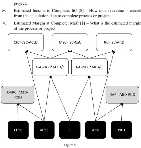
3.2.3 Financial (Attribute) Indicators
Measurement indicators:
i. Planned Cost to Date: PCtD [$] – Planned cost from the process or project start till the date of calculation.
ii. Actual Cost to Date: ACtD [$] – Money spent from the process or project start till the date of calculation.
iii. Planned Income to Date: PItD [$] - Planned revenue from the process or project start till the date of calculation.
iv. Actual Income to Date: AItD [$] - Actual revenue from the process or project start till the date of calculation.
Differentiation indicators:
i. Difference between Actual and Planned Cost: DAPC [$] – How much more or less cost was needed to the date of calculation.
ii. Difference between Actual and Planned Income: DAPI [$] – How much more or less revenue was earned to the date of calculation.
Prediction Indicators:
i. Estimated Cost at Complete: CaC [$] – Total cost of process or project.
ii. Estimated Cost to Complete: CtC [$] – How much cost is needed from the calculation date to complete process or project.
iii. Estimated Income at Complete: IaC [$] – Total revenue of the process or project.
iv. Estimated Income to Complete: ItC [$] – How much revenue is earned from the calculation date to complete process or project.
v. Estimated Margin at Complete: MaC [$] – What is the estimated margin of the process or project.
Figure 5 Financial Indicator Tree
Financial indicators can be applied as potential and effectiveness indicators. Table 3 gives some examples for interpretation.
Table 3
Interpretation of Timing Indicators by Focus Dimension Financial
Indicator
Focus / Potential Focus / Efficiency Focus / Effectiveness Planned Cost to
Date: PCtD [$]
Planned cost of inputs
N/A Planned cost of outputs
Actual Cost to Date: ACtD [$]
Actual cost of inputs
N/A Actual cost of outputs
Planned Income to Date: PItD [$]
N/A N/A Planned income of
outputs Actual Income to
Date: AItD [$]
N/A N/A Actual income of
outputs
4 Case Study
A middle sized Hungarian subsidiary of an international financial company started an operation development project aimed to optimize one of its core processes.
After analyzing the current state of operation, experts defined more than 200 development actions, which were handled as small projects. Despite that they had to produce different outputs, most of them had similar structure of activities:
planning tasks, developing, testing and implementing solutions. These small projects were considered the repetitive elements of the operation development program. This program was monitored by the FAR model.
Standard Measurement indicators were defined for all actions according to the FAR model. Table 4 shows these indicators, with actual and target values.
Table 4
Interpretation of Financial Indicators by Focus Dimension
FAR Indicator Interpretation of indicator in operation development program (examples)
Number of Opportunities for defect: O [No]
Defect types: missing information, unavailable resources, missing deadlines, unacceptable result.
Actual value: 4. Target value: N/A.
Number of Defects: D [No] No of defects for each type.
Actual value: according to measurement. Target value: 0.
Number of Defective Items:
DI [No]
Actions having defects as defined above.
Actual value: according to measurement. Target value: 0.
Correction Time per Defect: CTD [h]
Actual value was calculated for the four types of defects according to what kind of particular defect occurred:
Missing information: time of getting particular information
Unavailable resources: time of involving or replacing a particular resource
Missing deadlines: time of completing tasks linked to a particular deadline
Unacceptable result: time of correcting particular outputs
If multiple defects for a defect type occurred, average of correction time was calculated.
Target value was 0 for all defects.
Correction Cost per Defect:
CCD [$]
Actual value was calculated for the four types of defects according to what kind of particular defect occurred:
Missing information: cost of getting particular information
Unavailable resources: cost of involving or replacing a particular resource
Missing deadlines: cost of completing tasks linked to a particular deadline
Unacceptable result: cost of correcting particular outputs
If more than one defect in a defect type occurred, average of correction cost was calculated.
Target value was 0 for all defects.
Item at Complete: IaC [No] No of small projects.
Actual value: 210. Target value: N/A.
Number of Measurement Cycles Left: MCL [No]
No of weeks between calculation date and project finish date.
Actual value: according to measurement. Target value:
N/A.
Completeness of activities:
C [%]
Completeness of the whole project.
Actual value: according to measurement. Target value:
planned completeness.
Start Date of activity: SD [mm.dd.yyyy]
Start date of the whole project.
Actual value: real start date. Target value: N/A.
Planned Completeness Date: PCD [mm.dd.yyyy]
Planned date of current completeness of assessed small projects.
Actual value: planned date. Target value: N/A.
Actual Completeness Date:
ACD [mm.dd.yyyy]
Actual date of current completeness of assessed small projects.
Actual value: recorded date. Target value: planned date.
Planned Cost to Date: PCtD [$]
Cost of results and inputs of small projects according to its plan.
Actual value: planned cost. Target value: N/A.
Actual Cost to Date: ACtD [$]
Actual cost of results and inputs of small projects.
Actual value: according to measurement. Target value:
planned cost.
Planned Income to Date:
PItD [$]
N/A
Actual Income to Date:
AItD [$]
N/A
Actual values of indicators were measured and calculated on a weekly basis.
Values were recorded in Excel sheets. Each indicator had an information box with indicator name, unit, actual and target values and their qualifications marked by the following colors:
Red means the actual value is worse than target value
Green means the actual value is better than or equal to target value
White means that there is not a planned or actual value Parts of the indicator box are demonstrated on Figure 6.
Indicator name [unit]
Actual value Target value Color mark
Figure 6 Content of indicator box
Figure 7, Figure 8 and Figure 9 show the elements of one of the weekly reports of indicators with hypothetic values.
2800 0 300 000
140 0 0,024 0 2,222 0 15 000 0
5 0 12 0 4 N/A 0 0
0 0 0 0 210 N/A 0 0
10 0 8 0 9 0 1 500 0
0 0 0 0 20 N/A 0 0
CCD (mis. inf.) [$]
MCL [No]
QUALITY INDICATORS
DIFFERENTIATING INDICATORSPREDICTION INDICATORS
ETDaC [h] ECDaC [$]
IaC [No]
MEASURING INDICATORS
ETD [h] DPO DPDI ECD [$]
CCD (unav. res.) [$]
CCD (mis. dea.) [$]
CCD (unac. res.) [$]
O [No]
DI [No]
CTD (unac. res.) [h]
D (mis. inf.) [No]
D (unav. res) [No]
D (mis. dea.) [No]
D (unac. res.) [No]
CTD (mis. inf.) [h]
CTD (unav. res.) [h]
CTD (mis. dea.) [h]
Figure 7
Quality indicators in weekly report of the FAR model
432 360 324 252 04.08.16 01.27.16
10 0 108 N/A
25 30 02.01.15 N/A 05.10.15 N/A 05.20.15 05.10.15
MEASURING INDICATORS
DoC [mm.dd.yyyy]
C [%] SD [mm.dd.yyyy] PCD [mm.dd.yyyy] ACD [mm.dd.yyyy]
DIFFERENTIATING INDICATORS
DAPD [day] TSD [day]
TIMING INDICATORS
PREDICTION INDICATORS
TaC [day] TtC [day]
Figure 8
Timing indicators in weekly report of the FAR model
3000 2667 2 250 1867
-50 0 #HIV! N/A
800 N/A 750 800 25 30
C [%]
DIFFERENTIATING INDICATORS
DAPC [$] TSD [day]
MEASURING INDICATORS
PCtD [$] ACtD [$]
FINANCIAL INDICATORS
PREDICTION INDICATORS
CaC [$] CtC [day]
Figure 9
Financial indicators in weekly report of the FAR model
The FAR indicator structure included sub-indicators too, which were the interpretation of the project metrics for small projects. In addition, the actual values of these indicators were presented – among others - as run-charts, which helped management to assess the change of the values of the indicators, week-by- week.
Owing to the application of this structure, the management board was able to get detailed information about the progress of small projects, regularly, recognize the negative difference between actual and target values, define corrective activities and check the effects of their implementation.
Conclusions
Application of the FAR model proved its ability to monitor process or project activities and provide information about negative events and their effects. Due to its structure, management can recognize, in time, if there is something to be corrected regarding inputs, activities and/or outputs, from the perspective of quality, time and cost. Having information on the difference between actual and target values, the future values of indicators can be estimated. Further developments should focus on the application of the FAR model or any similar models for other types of projects and programs.
Aknowledgement
FAR model could not be elaborated and tested without the cooperation of the staff of Resultator Ltd.
References
[1] Breyfogle, F (2013): The Business Process Management Guidebook: An Integrated Enterprise Excellence BPM System, Citius Publishing
[2] Eilat, H. et al. (2008): R&D project evaluation: An integrated DEA and balanced scorecard approach, Volume 36, Issue 5, pp. 895-912, Omega:
The International Journal of Management Science
[3] Fleming, Q. W et al. (2000): Earned Value Project Management, 3rd Edition, Project Management Institute
[4] Kaplan, R. et al. (1996): The Balanced Scorecard: Translating Strategy into Action, Harvard Business Review Press
[5] Kim, Y. et al. (2010): Management Thinking in the Earned Value Method System and the Last Planner System, Volume 26, Issue 4, Journal of Management in Engineering
[6] Milis, K. et al (2004): The use of the balanced scorecard for the evaluation of Information and Communication Technology projects, Volume 22, Issue 2, February 2004, pp. 87-97, International Journal of Project Management [7] Papalexandris, A. et al. (2005): An Integrated Methodology for Putting the
Balanced Scorecard into Action, Volume 23, Issue 2, April 2005, pp. 214- 227, European Management Journal
[8] Paquin, J. P. et al. (2002): Assessing and controlling the quality of a project end product: the earned quality method, Volume: 47 Issue: 1, IEEE Transactions on Engineering Management
[9] Pyzdek, T. (2003): The Six Sigma Handbook, McGraw-Hill Companies, Inc.
[10] Vandevoorde, S. et al. (2006): A comparison of different project duration forecasting methods using earned value metrics, Volume 24, Issue 4, May 2006, pp. 289-302, International Journal of Project Management
[11] Yong-Woo Kim et al. (2000): Is the earned-value method an enemy of work flow, Eighth Annual Conference of the International Group for Lean Construction (IGLC-8)