An Alternative Method in Optimizing Random Outcomes

An Alternative Method in Optimizing Random Outcomes

Sándor Molnár

¹

, Ferenc Szidarovszky

²

1 Institute of Mathematics and Informatics, Szent István University, Páter K. u. 1, H-2100, Gödöllő, Hungary, molnar.sandor@gek.szie.hu

2 Ferenc Szidarovszky, Department of Applied Mathematics, University of Pécs, Ifjúság u. 6, H-7624, Pécs, Hungary

Abstract: Within economic literature random outcomes can be characterized by their certainty equivalents. In this article, a general approach for their extension is first outlined and then special cases are shown. The two most simple of these cases result in the classical formula of certainty equivalent, and by increasing the degree of the approximating Taylor polynomials, more advanced formulas are derived. Additionally, a simple advanced formula is compared favorably to the classical approach in a computer study and some application models are discussed to illustrate the methodology.

Keywords: decision making; uncertainty; applications

1 Introduction

In practical decision making problems we often face random elements due to modeling, natural and economic factors. In constructing mathematical models certain elements are neglected in order to keep the model solvable. The natural and economic components are usually uncertain due to the lack of relevant data and prediction errors. Uncertainty in mathematical models is usually formulated with fuzzy or stochastic methodology, where the uncertain quantities are considered fuzzy numbers with appropriate membership functions or as random variables with certain probability density functions which are only estimated so there is no way to construct theoretically correct function forms. The fuzzy methodology constructs a fuzzy number as the solution, which is then defuzzified, for which several alternative methods are available [6, 1]. If stochastic methodology is chosen, then stochastic programming [5, 11] is a very popular approach. In order to decrease uncertainty, the variances of the objective functions are minimized in addition to optimizing the expected values of the objectives leading to multi-objective optimization problems [13, 10]. Data analytical methods also can be used to reduce variances [7]. Bayesian methodology [3] is

based on the repeated updating of the probability distributions using new sample elements. In the economic literature very often certainty equivalents are introduced and optimized instead of random objectives [12]. They are linear combinations of expectations and variances, which is the same as applying the weighting method.

There are many applications of the stochastic methodology including extractibility of natural resources [2], groundwater management [4], emission allowance prices [9], reliability engineering [8]. The many application fields show the importance of this methodology.

In this paper an alternative approach is introduced, which can replace the certainty equivalent and provides more accurate solutions. The authors of this paper could not find any earlier work deriving more advanced solutions and relating them to the root locus method. After the theoretical issues are discussed, a comparison study is reported and some particular models are described to illustrate the methodology. The last section is devoted to conclusions and future research directions.

2 The Mathematical Methodology

Consider a random variable

x

representing the value of an outcome. The goodness of the different values of

x

is characterized by a utility function

u (x )

. Introduce the notation xE(x) and



² Var(x). Clearly the random outcome can be replaced by a deterministic value

x

^, such that

 u x  u x f x dx E

x

u ( ) ( ) ( ) ( )









^{ } 

^(2.1)

where f(x) is the probability density function of

x

. If u(x) is strictly monotonic, then

. ) ( )

1

(

 



 

 











^u  ^{u x f x dx}

x

(2.2)

This formula cannot be applied in most cases, since

f (x )

is usually unknown.

We can however derive an acceptable estimate of

x

^ as follows. By the Taylor's formula

) ( )

)(

! ( ) 1 )(

( ) ( )

(

⁽⁾ ₁

2

x R x x x i u x

x x u x u x

u

^{i i} _m

i m











 



 

^(2.3)

and

) ( )

)(

! ( ) 1 )(

( ) ( )

(

^{( )} ₁

2

x R x x x j u x

x x u x u x

u

^{j j} _n

j n











       

^(2.4)

when

R

_m1

( x )

and

R

_n1

( x )

are the remainder terms. By omitting the error terms and taking expectation,

  ^{( ) ,}

! ) 1 ( )

(

⁽⁾

2

i i i

m

M x i u x

u x u E









^(2.5)

so (2.1) implies

i i i

m j j j

n

M x i u x

j u ( )

! ) 1

! (

1

₍₎

2 )

(

1 





 ^{ }

^(2.6)

where

M

i

 E  ( x  x )

ⁱ



is the

i

^th central moment of

x

and

  x

^

 x

. Notice that (2.6) gives an

n

^th degree polynomial equation for unknown



^{, from}

which

x

^

   x

. In order to find the right root of (2.6) consider the root loci of equation

, )

! ( 1

( ) 1

K x

j u

j j j

n

 



 ^(2.7)

where K is the parameter. Each locus shows how the associated root of this equation varies as the value of K changes. In the deterministic case

x  x

with

,

2 0



so K 0 and in this case

x

^

 x

implying that 0. Therefore, we have to select the locus which passes through the origin. The value of this locus at

i i i

m

M x i u

K ( )

! 1

()

2





(2.8)

gives the value of



.

Some special cases are presented next.

Example 2.1 Assume

m  n  1

, then we have

0 ) )(

(  

 x x

^

x

u

(2.9)

and if

u  ( x )  0

, then

x

^

 x

.

Example 2.2 Let

m  2

and

n  1

, then equation (2.6) becomes

)

2

2 ( ) 1

( x u x 

u    

(2.10)

implying that

2

) ( 2

)

( 

x u

x u



 



^(2.11)

so

2 1^

 x  

x

(2.12)

is the approximation of

x

^ with

) . ( 2

) (

x u

x u



 



^(2.13)

It is the well known certainty equivalent.

Notice that this method cannot be used if u

'

(x)0. Example 2.3 Let now

m  n  2

, then

2

2

( )

2 ) 1 2 ( ) 1

( x u x u x 

u       

(2.14)

or

.

2

0

2

   

 



(2.15)

If



²

 0

, then there is no uncertainty, so

  0

is the solution. In general,





 2

4 1

1  

^{2 2}

 











x x

x

(2.16)

and since at



²

 0

the solution has to be

x

, the positive square root has to be considered:





 2

4 1

1

^{2 2}

2





 





x

x

(2.17)

is the approximation of x by the more accurate method. ^

Similarly to the previous example this formula cannot be used if u

'

(x)0. If ,

0

 then 0, so

x

^2

 x .

3 Comparison Study

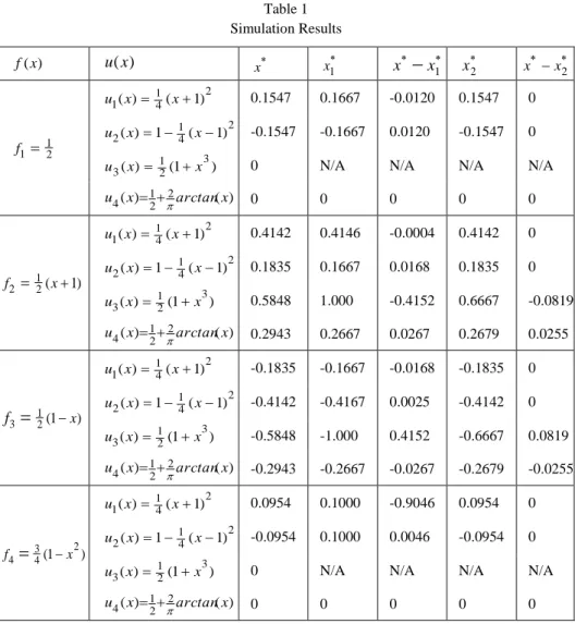
In order to compare the accuracy of formulas (2.12) and (2.17) we conducted a simulation study. Random variable

x

was considered with four different density functions on

[ 

1,1

]

as follows:

) 1 ( 4 ) 3 ( and ) 1 ( 2 ) 1 ( ), 1 ( 2 ) 1 ( , 2 ) 1

( _{2 3 4} ²

1 x f x x f x x f x x

f       

where

f

₁

( x )

is constant,

f

₂

( x )

is increasing,

f

₃

( x )

is decreasing and

f

₄

( x )

is mound-shaped. Four different utility functions were chosen,

), ( 2tan 2 ) 1 ( ), 1 ( 2 ) 1 (

, ) 1 ( 4 1 1 ) ( , ) 1 ( 4 ) 1 (

1 4

3 3

2 2

2 1

x x

u x x

u

x x

u x x u

 



















where

u

₁

( x )

is convex,

u

₂

( x )

is concave,

u

₃

( x )

is convex for x0 and concave for x0, and

u

₄

( x )

is convex for x0 and concave for x0. So a large variety of density and utility function types were considered, and 1644 cases examined. In each case the true value of

x

^ was determined based on equation (2.2), since both u(x) and f(x) were known for all cases. Table 1 shows the results. The first and second columns specify the density and utility functions, the third column shows the true value of

x

^. The fourth column gives the results based on (2.12) where

x

and ² are computed based on the given density functions. The sixth column contains the results obtained by using (2.17).

The fifth and seventh columns show the errors of the obtained estimates. Among the 16 cases we can find 10, where (2.17) gives the exact answer, in 4 cases (2.17) has smaller error, and in 2 cases the formulas could not be used.

If the utility function is linear or quadratic, then with nm2, 0

) ( )

( ₁

1  _ 

 x R x

R_{m n} in equations (2.3) and (2.4), so formula (2.17) is exact. In the cases of densities f₁ and f₄

,

(x)x0, furthermore ₃ ²

2

)

3

( x x

u  

which

is zero at x0, so formulas (2.12) and (2.17) cannot be applied. In addition



²



²

4

1 ) 4 (

x x x

u 

 



 with zero value at x0, therefore in the cases of densities f1 and f₄,  0 implying that x₁^ x₂^ 

x 

0 from both formulas (2.12) and (2.17).

Table 1 Simulation Results )

(x

f u(x) _x^{ }

x1 x^



x₁^ x^₂ x^x₂^

2 1 1 f

2 4 1 1(x) (x1)

u 0.1547 0.1667 -0.0120 0.1547 0

2 4 1 2(x)1 (x1)

u -0.1547 -0.1667 0.0120 -0.1547 0

) 1 ( )

( ₂^{1 3}

3 x x

u   0 N/A N/A N/A N/A

) ( )

( ²

2 1

4 x x

u  _arctan 0 0 0 0 0

) 1

2(

1

2  x

f

2 4 1 1(x) (x1)

u 0.4142 0.4146 -0.0004 0.4142 0

2 4 1 2(x)1 (x1)

u 0.1835 0.1667 0.0168 0.1835 0

) 1 ( )

( ¹₂ ³

3 x x

u   0.5848 1.000 -0.4152 0.6667 -0.0819

) ( )

( ²

2 1

4 x x

u  _arctan 0.2943 0.2667 0.0267 0.2679 0.0255

) 1

2(

1

3 x

f





2 4 1 1(x) (x1)

u -0.1835 -0.1667 -0.0168 -0.1835 0

2 4 1 2(x)1 (x1)

u -0.4142 -0.4167 0.0025 -0.4142 0

) 1 ( )

( ¹₂ ³

3 x x

u   -0.5848 -1.000 0.4152 -0.6667 0.0819

) ( )

( ²

2 1

4 x x

u  _arctan -0.2943 -0.2667 -0.0267 -0.2679 -0.0255

) 1

( ²

4 3

4 x

f





2 4 1 1(x) (x1)

u 0.0954 0.1000 -0.9046 0.0954 0

2 4 1 2(x)1 (x1)

u -0.0954 0.1000 0.0046 -0.0954 0

) 1 ( )

( ¹₂ ³

3 x x

u   0 N/A N/A N/A N/A

) ( )

( ²

2 1

4 x x

u  _arctan 0 0 0 0 0

4 Applications

In this section some application models are introduced.

Model 4.1 (Budget allocation) An investment firm with budget

B

has

n

investment opportunities, where opportunity

k

gives profit



_k per each invested dollar with E( _k) _k and Var(_k)_k². If the profits are independent, then

the expectation and variance of the profit _{k k}

k n

 x



1

 

from the total investment

k k

n

x x

1

 

are given as

 

_{k k}

k n k k k

n

x x

E

E   



1 1

) (







 ^



 (4.1)

and

 

^{2 2}

^,

1 1

2 Var( ) Var _{k k}

k n

k n

k

x

kx





 







 ^





^(4.2)

where x_k gives the allocated investment in opportunity k.

By assuming the utility function

u (  )  

² we have

u  (  )  2 

and

2 )

( 

 

u

showing that

  2

 1 , the objective function becomes

, 1

4 4 1 1 1 2

4 1 1

2 2 2 2

2 2 2

2















 

 



 



























 



 

(4.3)

so the firm solves the quadratic programming problem maximizing

2 2 1 2

1

k k k

n k k k

n

x

x 









   ^

 





subject to

B x

n k

x

k k n k









1

) , , 2 , 1 (

0 

(4.4)

Model 4.2 (Oligopoly

#

1) Consider an

n

-firm single product oligopoly without product differentiation. Let

x

_k be the output of firm

k

,

c

_k

( x

_k

)

its cost function.

The industry output is _k

k n

x x

1

 

, and the corresponding unit price function is

) (x

p

. However the firms do not know the exact price function, so firm

k

believes that the price function is

p

_k

( x )  

_k, where

p

_k

(x )

is the believed price function by firm k (usually different than the true price function) with a random error term _k resulting from market uncertainties. So firm

k

believes that its profit is



_k

( )

_k



_k

(

_k

),

k

k

 x p x    c x



(4.5)

which is considered as the random outcome for firm k.

By assuming that

E ( 

_k

)  0

, Var(_k)

 s

_k², we have

 

_{k k k}

( )

_k

(

_k

)

k

 E   x p x  c x



(4.6)

and

2

.

2

2 Var( _k) _{k k}

k



 

s x



^(4.7)

If the firms select exponential utility functions,

^u

k

 

k

^e

^{k k}

^,



 

 then

2

k k

 



is constant for each firm, so the objective functions become

.

2 4 1 ) 1

( ) ( 2

4 1

1 ^{2 2 2 2 2 2}

k k k k k

k k k k

k k k k

x x s

c x p x x s







       ^{  }

 (4.8)

Notice that this is the profit function (4.5) of oligopolies without uncertainty and product differentiation where the modified cost functions are

.

2 4 1 ) 1

(

2 2 2

k k k k k

k

x x s

c 







 (4.9)

Model 4.3 (Oligopoly

#

2) Consider now an oligopoly when the firms know the true price function p(x) but their costs are uncertain. Assume that because of uncertain prices of labor, energy and material firm

k

believes that its cost function is

c

_k

( x

_k

)  

_k

( x

_k

)  

_k

x

_k, where



_k

( x

_k

)

is a known function and



k is a random variable with E

( 

_k

)  0

and Var

( 

_k

)  s

_k². Notice that



_k is a random term in the marginal cost. The profit of firm k is its random outcome. The expectation and variance of the profit of firm

k

is

) ( )

(

1

k k l l

n k k

k

E  x p x  x

   

 



 





 ^(4.10)

and

. )

(

Var

^{2 2}

2

k k k

k

   s x



(4.11)

where





 

  

 l l

n

x p

1

is the price function which is considered to be a public information for the firms. Similary to the previous case (2.17) gives the modified objective function of firm

k

:

.

2 4 1 ) 1

(

2 2 2

1 k

k k k k

k l l

n k

x x s

x p

x 

    









 

  

 (4.12)

If the utility functions u_k(_k) are exponential, then _k is a constant for all firms.

Conclusion

A well-known concept of the certainty equivalent is replaced by a general approach, which can be reduced to the certainty equivalent in a very special case.

A simulation study showed the advantage of the new approach resulting in more accurate approximations.

The methodology was illustrated on three simple models. The more accurate formulas are based on higher order Taylor polynomials of the utility function.

Methods (2.12) and (2.17) are based on the adjustment constant



which depends on the first two derivatives of the utility function. Its special form implies two important facts. If

u 

(x)0, then  cannot be determined, so these methods cannot be used as was shown in two cases of Table 1. If

u 

(x)0

,

then 0 implying that x^



x, which was also shown in two cases of the utility function

)

4(x

u

. In our comparison study we found no case when the classical certainty equivalent was better than our improved formula. We expect that by selecting higher order Taylor polynomial approximations of the utility function the accuracy of the resulting formulas can be improved even further.

Higher order formulas can be used in cases when lower order formulas cannot be used.

In our future research higher order approximations (with larger values of

m

and

n

) will be used in particular applications which will be selected from broad fields of engineering and economics.

References

[1] Bellman, R. and Zadeh, L. A. (1970): Decision Making in a Fuzzy Environment, Management Science 17(4), pp. 141-164

[2] Csábrági, A., Molnár, M. (2011): Role of Non-Conventional Energy Sources in Supplying Future Energy Needs, Bulletin of the Szent István University, Gödöllő

[3] DeGroot, M. H. (1970): Optimal Stochastic Decisions. New York:

McGraw-Hill

[4] Hatvani, I. G., Magyar, N., Zessner M., Kovács, J., Blaschke, A. P. (2014):

The Water Framework Directive: Can More Information Be Extracted from Groundwater Data? A Case Study of Seewinkel, Burgenland, Eastern Austria, Hydrogeology Journal 22(4), pp. 779-794

[5] Kall, P. and Wallace, S. W. (1994): Stochastic Programming. Chichester:

Wiley

[6] Klir, G. J. and Yuan, B. (1995): Fuzzy Set and Fuzzy Logic: Theory and Applications. Upper Saddle River: Prentice Hall

[7] Kovács, J., Kovács, S., Magyar N., Tanos, P., Hatvani, I. G., Anda, A.

(2014): Classification into Homogeneous Groups Using Combined Cluster and Discriminant Analysis, Environmental Modelling & Software 57, pp.

52-59

[8] Matsumoto, A., Szidarovszky, F. and Szidarovszky, M. (2014):

Incorporating Risk Economic an Optimization Model of Reliability Engineering, International Journal of in Behavior and Organization 3(1-2), pp. 1-4

[9] Molnár, M. (2014): Opportunities for Hungary under the Stability Reserve of the EU ETS, Journal of Central European Green Innovation 2(2), pp.

105-114

[10] Molnár, S., Szidarovszky, F. (2011): Game Theory, Multiobjective Optimization, Conflict Resolution, Differential Games (in Hungarian) Budapest: Computerbooks

[11] Prekopa, A. (1995): Stochastic Programming. Dordrecht: Kluwer Academic Publishers

[12] Sargent, T. J. (1979): Macroeconomic Theory. New York: Academic Press [13] Szidarovszky, F., Gershon, M. and Duckstein, L. (1986): Techniques for

Multi-objective Decision Making in Systems Management. Amsterdam:

Elsevier

[14] Szidarovszky, F. and Yakowitz, S. (1978): Principles and Procedures of Numerical Analysis. New York: Plenum Press