Decision Support Methods and Systems /Practical Workbook/

Decision Support Methods and Systems

/ Practical Workbook /

Decision Support Methods and Systems / Practical Workbook/

Written by:

Tibor Pupos

University of Pannonia Georgikon Faculty Gábor Pintér

University of Pannonia Georgikon Faculty (1.5; 2.4)

Edited by:

Tibor Pupos

Reviewed by:

András Tölgyes

Translated by:

Arnold Gór Erika Kiss Győriné

University of Debrecen, Centre for Agricultural and Applied Economic Sciences • Debrecen, 2013

University of Debrecen Faculty of Applied Economics

and Rural Development

University of Pannonia Georgikon Faculty

© Tibor Pupos, 2013

Manuscript finished: August 31, 2013

ISBN 978-615-5183-91-1

UNIVERSITY OF DEBRECEN CENTRE FOR AGRICULTURAL AND APPLIED ECONOMIC SCIENCES

This publication is supported by the project numbered TÁMOP-4.1.2.A/1-11/1-2011-0029.

Table of contents

Foreword 5

1 The decision as a management function ⁶

1.1 Edit the decision matrix and the quantification of its elements 7 1.2 Select strategic version under uncertain decision-making conditions 10 1.3 Choosing strategic version between risky conditions 12

1.4 Application of the decision tree 14

1.5 The role of the utility functions in the decision-making 16

1.6 Application of the method KIPA 23

2 The methods and procedures used on tactical and operational level ³⁸

2.1 Application of the LP model 38

2.1.1 Compilation of food portion in a dairy farm 38

2.1.2 Optimization of a fodder mixing plant‟s ware transportation 45 2.1.3 Scheduling of production, optimization of finished goods 49

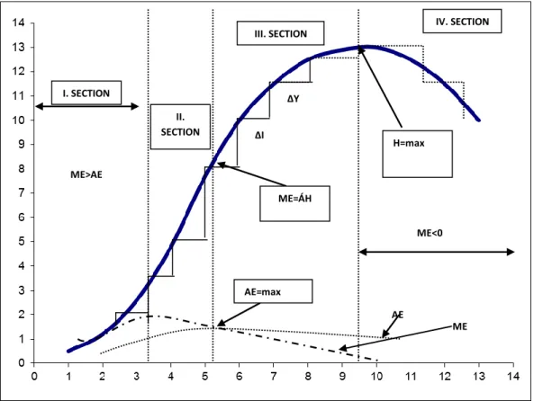
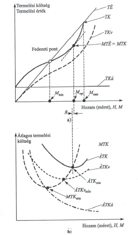
2.2 The application of production and cost curves 55

2.2.1 The questions related to production theory 55

2.2.2 Defining fertilizer doses with production and cost functions 61

2.3 The optimization of stock management 64

2.3.1 The important relationships of stock management 65

2.3.2 The cost stockholding 69

2.3.3 Theoretical basics of stocking policies 72

2.3.4 Resource management models 74

2.3.4.1 The model of optimal (economic) order quantity (EOQ) 75 2.3.4.2 The stock keeping ratio, as the central element of the

EOQ model

77

2.3.4.3 The use of stochastic models 80

2.4 The Graph theory and its application 84

2.4.1 The creation of a Gantt-chart based on the example 85 2.4.2 Creating activity on arrow (CPM) on a given example 89 2.4.3 Activity on node network drawing based on an example 99 2.4.4 Managing risk elements int he network /PERT/ 109

2.5 Break even principle and its application 116

2.6 The selection between investment alternatives 122

2.6.1 The indicators of an investment‟s efficiency and cash flow estimation

122 2.6.2 Decision between the investment alternatives 125 2.6.3 The connecting questions of cash flow and structure of sources

(liabilities)

126

Bibliography ¹³⁰

Appendix ¹³¹

Foreword

Ongoing changes in the factors of the management system affecting the condition of businesses so we can say they are under constant pressure to adapt. Long-term survival largely dependent on the extent of how effectively adapt to these changing conditions. It is envisaged that the successful adaptation requires a strategy that can respond quickly and successfully to changes. The response, for “What's next?”, answer to questions which required professional decisions and, what is very important in present, fast decision making, at each hierarchy - strategic, tactical and operational - level.

It is clear for us that effective adaptation is important requirement for the agricultural corporations and their leaders with decision-making competence. If we add the well-known sectorial features that adjustment latitude - where applicable - substantially curtailed, we can say that these decision-makers are in more difficult position than the decision-makers in other areas, sectors. Therefore, the agricultural professionals can not work without those methods and procedures which contribute to the professional decisions-making and quantifying the effects of changing conditions. These can therefore justify the discussion of the related knowledge.

Can not be argued - in line with the development of certain disciplines - that we would be constrained in various methods. However, it can be stated that the sectorial specificities in many cases significantly change or exclude the applied methods, procedures which are used effectively in other areas of production - e.g. industrial production. Therefore, the knowledge in this book is basically focusing the application of decision support methodologies in the agricultural sector. So the focus in the discussion of this knowledge is the applicability of certain methods in agriculture - and not the theoretical background of the method.

It is important also to point out that the use of certain techniques can only be unsuccessful without professional knowledge, the result is sure to be failure. Not all the related professional knowledge are discussed in detail, reference is made only for the most part. If the necessary technical knowledge is not active for those concerned, they should make it so in literature, and by looking at their notes. Those areas were selected in which the characteristics of the agricultural production do not create barriers for the application of the discussed methods. We always review the theoretical knowledge which are required for the practical application of some methods, facilitating the application of the method to learn. To deepen the knowledge and to learn skill level of this, we state additional examples.

Keszthely, 2012

The Authors

1. The decision as a management function

It is known, that the operation of a company (as an economic system) must not be incidental.

For rational functioning, management and regulatory processes are required. The interpretation of concepts and categories of this knowledge is not considered uniform because different understanding of various academic schools lies behind them, closely related to their development. In addition, the evolution of co-science - company theory, systems theory, etc. - the practice of different countries, the use of language is also reflected in the related these concepts and categories. The governing is considered as the most general concept. The leadership, administration, organizational concepts are organizations related and express the narrower sense of the management.

Governance: In a general it means the intervention of processes in order to achieve some goal. Governing is needed because the balance of the system is disrupted by changes in the interaction between the system and its environment. Thus, the system responds to environmental changes for a specific system state. (Example: when the gas prices rise, the house insulation is a rational action or the solar energy use for hot water preparation, etc).

Governance is based on pressure and back pressure between system and its environment. The governance processes focus on targeted interventions. With this intervention the leadership or administration processes influence the whole system. To start the governance process, namely the intervention process, the decision is required.

Decision: It means, in general, to select a set of options or the only option from a subset of options.

When we make a decision, we always find ourselves facing to the so-called decision problem.

It is therefore appropriate to look the elements of the decision problem. These are summarized below.

1. Actions (activities) 2. Events

3. Probabilities of the events occurrence*

4. Results (outputs) 5. Decision criteria*

6. Individual preferences*

* These elements are highly dependent on the decision maker, because the choice of probability judgment and decision criteria is highly dependent on the decision-maker.

The decisions can be classified according to several criteria. For a certain decision the probability of an event is 100%. When uncertain decision occurs, the outcome of the options for action is impacted by such interferences influence, which occurrence or the extent of the impact may not be related probabilities. Risky decision is when the disturbance occurrence probabilities are known or considered to be known to a personal decision (This interpretation of probability is called subjective probability). The analysis usually is determined by the

relative frequency. The concept of objective probability associated with this. In this context, the objective probability is considered a relative frequency effect (infinite).

Decisions are made on specific dates, extend to a specific period (which is a finite period) so it is not possible to perform an infinite number of experiments, and the conditions on the process can not be considered recurrent. Therefore the "objective" probabilities can not be used in decision making. What is relevant is the decision maker believes in the events occur, what is influenced by several factors, e.g. the decision-makers attitude, experiences, position, etc.

1.1 Edit the decision matrix and the quantification of its elements The target of the decision matrix is to express and summarize those numerical results and the actual conditions that affect them which are needed for the decision making. The decision matrix elements are included in the first table.

Table 1: The decision matrix structure

Actual conditions, events Actions, options for action

A1 A2 An

T₁ E11 E12 E1n

T₂ E21 E22 E23

Tn En1 En2 Emn

The actions, options for action mean the strategic variants, the decision-maker must choose from them. Symbols:

A1 A2 An

The actual conditions, events affect the outcome of the actions, depending on the value of the random coefficients of their occurrence. Symbols:

T1 T2 Tm

The results (outputs) are numerical values for specific actions and actual situation. Symbols:

E₁₁ E₁₂ E_mn

The economic substance of the outcomes of actions and actual conditions can be the gross margin, accounting income categories, economic profit, etc. It can be seen that the numerical values of the output depending on the variable of strategic options and the actual conditions.

Keep track what was said through an example.

TASK: We accept the following. A group of investors, in an area with very rich natural values, trying to achieve investment for plant protection service. The three prospective owners are well-prepared professionals, their professional qualities are well known not only in the small region. But as decision makers, they have significantly different risk-taking willingness, mentality and decision-making experience. One of them - Jenő – is more risk-taking, gamble, have lot of decision-making experience. Berci is more risk-averse than risk-taking type. Benő likes the certain things, he is a cautious, very prudent type, clearly can be called risk-averse.

Based on preliminary surveys, a number of individual farmers, small businesses, SMEs and business organizations with over 2500 ha of arable land, has also indicated the need for the service. The Ltd. would provide complex plant protection services, giving priority to precision plant (crop) protection technologies. The preliminary survey is not exhaustive. In this context, the changes in demand is an important risk factor in terms of the return on investment, that significantly impact on returns on investment of the profit side through the development of the capacity utilization of resources. They agreed on the need to develop a decision matrix. It should also be noted that due to the distribution of the local enterprises in this small area, the service unit price can move between 3,100 - 3,300 Ft/ha. Higher fees could not be validated over the upper limit of the service price. Due to the information on the needs and the owners risk taking ability differences the following strategic variants come to mind as possible substance of the decision matrix:

Options for action: Because of the pricing strategy and the risk taking willingness of the owners the following strategic variants come to mind:

A1: Service price 3100 Ft/ha A₂: Service price 3200 Ft/ha A3: Service price 3300 Ft/ha Expected conditions:

T1: Capacity utilization 60%

T₂: Capacity utilization 75 % T3: Capacity utilization90 %

The quantification of the results we take the values based on 2nd table.

Quantify the output values of the decision matrix. Quantification of the algorithm of E11and the results are included in the 3rd table is.

Table 2: Possible amounts for the quantification of the strategic variations

Appellation Unit Amount

Equipment acquisition costs thousand Ft 27600

Depreciation rate % 14

Property acquisition costs thousand Ft 2000

Depreciation rate % 4

Unit cost of service

- Wages + public charges Ft/ha 222

- Material and material-type expenses

Ft/ha 1006

Insurance, tax thousand

Ft/year

140

Rates of return on alternative investments % 4

Maximum price of service Ft/ha 3500

T1 % 60=2280 ha

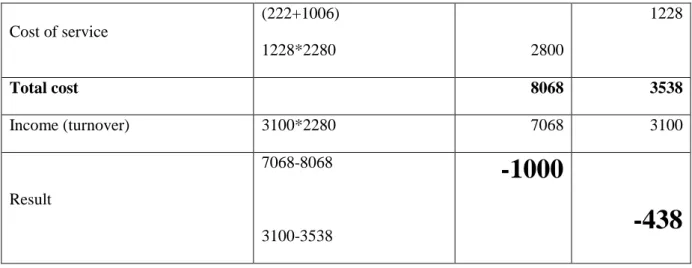
Table 3: The quantification algorithm of E11

Appellation Algorithm

Total Unit

thousand Ft Ft/ha

Buildings

2000*0,04 (2000*0,04):2280

80

35

Equipment

27600*0,14 (27600*0,14):2280

3864

1695

Insurance, tax 140:2280 140 61

Permanent total 4084 1791

Alt. Return on investment

29600*0,04 (29600*0,04):2280

1184

519

Fixed costs in total 5268 2310

Cost of service

(222+1006)

1228*2280 2800

1228

Total cost 8068 3538

Income (turnover) 3100*2280 7068 3100

Result

7068-8068

3100-3538

-1000

-438

INDEPENDENT TASK: A detailed breakdown of the result of E12 (in the decision matrix) and the solution and deliver by deadline. (Use Table 3).

The results of each action and actual states are summarized in the decision matrix (Table 4).

Table 4: Investment decision-making matrix

Actual conditions, events

Actions, options for action

Sign

Capacity utilization

% - ha

A1 A2 A3

T1 60 - 2280 -1000 -772 -544

T2 75 - 2850 67 352 637

T3 90 - 3400 1097 1437 1777

The results show that how develop the intended results depending on the capacity utilization and the price. Because the price and the service unit variable cost are fixed (varies in proportion), the standard deviation of the results is moved by the capacity utilization.

1.2. Select strategic version under uncertain decision-making conditions Several principles available that can be used for decisions which give professional support in uncertain decision-making situation to justify it. Obviously, the decision-maker takes a decision by one principle. On this basis with this decision the strategy, actions or activities are also chosen. That strategy is different from that which would be chosen based on another principle or criteria. The selection of the criteria should not be given general guidance in the decision-making subjectivity plays a decisive role. In taking decisions, the uncertainty plays

an important role in the decision matrix, allows to select the best alternative formalization of actions, depending on the chosen decision criterion:

Laplace-Criterion: Since we do not know the probability of occurrence of the actual status, those should be regarded as equal. It follows that, on this criterion, the best decision and action program will be, the result of which is the largest. So the actual states equally third likely to be taken into account. On this basis, the T₃ actual state will be accepted and action A₃ is selected as a quantitative indication with the biggest decision criterion for choosing category (income).

Maximin-Criterion: from the action alternatives that one is considered preferable which have the worst possible outcome is the smallest compared with the other options. The worst results are - understandably - in the T1 condition, which occurs when the capacity utilization is 0%. (- 1000, -772, -544). Among them, the best one is selected, so that A3.

Maximax-Criterion: In contrast to the previous one when the decision is made on the basis of this criterion, we choose the best alternative result from the probably highest results (T₃ and A3, which is 1777 thousand HUF). This principle is used by the optimist decision-makers.

It is important to point out that if there is a decision-making situation, when the costs or the loss is to be reduced, minimized, the last two principles must be interpreted in the opposite sense.

Minimum regret principle:

You must select the action for which the minimum amount should resign (compared to the highest possible) if the worst occurs from the events. Better understand the application of this principle if we transform the decision matrix to regret-matrix. The conversion is that we calculate the deviations to the results of actual status for every version and these results are written in the appropriate line of the column. (Table 5)

Table 5: Investment of the regret matrix Actual conditions,

events Actions, options for action

sign

Capacity utilization

% - ha

A1 A2 A3

T1 60 - 2280 -456^* --228 0

T2 75 - 2850 570^* 285 0

T₃ 90 - 3400 680^* 340 0

In the case of a 90% capacity utilization the best result is 1777 thousand HUF. Extract from this result the results of the two actions. So

(1777-1097= 680; 1777-1437=340;1777-1777=0 )

The 75% of capacity utilization results with the best 637 thousand HUF. Accordingly this, due to

(637-67=570; 637-352=285; 637-637=0)

The actual condition of 60% capacity utilization results with the best action of -544 thousand HUF. Thus tend

(-544-(-1000) = -456; -544-(-772)= -228; -544-(-544)=0)

It follows that the zero matrix elements are the most favorable outcome, the values of the options, and the remaining elements of the matrix are expressed in relation to it. Values marked with stars indicate the greatest differences in values, so if this principle is enforced, then the "least regret" is selected from the lowest value marked with star, so the A1 action.

Hurvitz-Criterion: This is a transition between the maximax and maximin principles. The typical decision-makers relate differently in different decisions, with varying degrees of optimism, etc. If this criteria the decision-maker's optimism are quantified using optimism coefficient (α-alpha), on 0-1 scale. The optimistic decision-maker‟s α coefficient is closer to 1, the pessimist‟s is closer to 0. By this we correct the results of each alternative. So, the best result is multiplied by α, however, the minimum result is multiplied by (1 - α). That strategy has to be chosen in which the maximum amount received. So

FH_k =

α

α

FH_k = Adjusted results of actions E = Best result of actions e = Worst result of actions

You have to choose the action with the highest corrected results compared with other corrected results. Accept the value of α is 0.7. The corrected results are as follows.

Adjusted results of A1 action: (1097 * 0,7) + (-1000 * 0,3) = 770 + -300 = 470 Adjusted results of A2 action: (1437 * 0,7) + (-772 * 0,3) = 1006 + -232 = 774 Adjusted results of A₃ action: (1777 * 0,7) + (-544 * 0,3) = 1244 – 163 = 1081 Based on the corrected results A3 should therefore be chosen.

Selection of the criteria listed above can only be done on intuitive basis. The selections of the criteria are highly dependent on the decision maker. It will be appreciated that other criteria

can be chosen by an optimist, a prudent or a conservative decision-maker. However, none of these cases can be called perfect, but one of them as normative rule should be adopted and consistently applied.

1.3. Choosing strategic version between risky conditions

The risky decisions, we have the random coefficients of the occurrence of actual states and their numerical values. These values describe the random variables stochastic or random

"behavior". The probability calculations, the following rules shall be observed:

 The probability (symbol: P) is between 0 and 1.

 The entire event system (actual state random coefficients sum) = 1.

 The probability of occurrence of two or more mutually exclusive events is equal to the sum of each probability.

 The probability of occurrence of two or more mutually exclusive events is equal to the multiplication of the individual probabilities.

The random coefficients measure the risk. The multi-faceted risk perceptions take into account the objective and subjective elements. The behavior of the random variables is characterized by mathematical functions. The function can be continuous or discrete.

For several reasons, the continuous random variable is treated as a discrete value. The representation of the values of the random variables are used the following

 Distribution function

 Cumulative density function

 Frequency histogram

 Other display modes.

These modes of procedure used subjective probability estimation. The methods which are used in risky decision-making process are described below.

 Decision-making matrix

 Decision Tree

 The use of utility functions.

Decision matrix between risky conditions

The decision matrix for risky decision-making processes can be used with some supplements.

The additions are known to use random coefficients, as follows:

Actual conditions, events

Random coefficient

T₁ p₁ 0,70

T2 p2 0,20

T₃ p₃ 0,10

An important rule is that the actual states must be exhaustive and mutually exclusive.

Consequently, the sum of the random coefficients is 1. In the example, the actual conditions are mutually exclusive each other, so the requirement for their joint probability is satisfied, because 0.7 + 0.2 + 0.1 = 1

Despite the continuity of the event variables, it is convenient to handle as discrete variables.

Modes of procedure might include.

Expected rate principle: we quantify the expected values, so the results are multiplied by the random coefficients. We select the action for which the total expected value is the maximum.

In accordance to the explanation, the expected values can be found in Table 6 T1 actual condition: 0,7 * -1000 = -700 (T1A1)

T2 actual condition: 0,2 * 67 = 13 (T2A1) T₃ actual condition: 0,1 * 1097 = -110 ( T₃A₁)

Table 6: The decision matrix with the expected values

Actual conditions,

events

Random coefficient

Actions, options for action

A1 A2 A3

T1 0,70 -700 -540 -381

T₂ 0,20 13 70 127

T3 0,10 110 144 178

Total 1,00 -577 -326 -76

We do not have to prove that the decision making problems in the practical life are more complex, due to the diversity of conditions which have impact to the result and they occurs regardless of the decisions. These conditions are independent of each other, but also may affect each other. For example, the input price increase will affect the price of fuel. It may cause service fee and price rise. However, the price increase may be associated with a drastic reduction in planned capacity, etc. Thus the method makes it possible to take into account a variety of events, and the event can be corrected by the probability of a new event. In this case the results are corrected by the combined probability value of the coefficient. If we assume that the labor force and machinery operating costs - because of the rise in prices - 10%, the probability of occurrence is 80% than the combined random coefficient:

T1 = p1 x pprice = 0,70 x 0,8 = 0,56

Important to note that due to the planned increase in prices the results have to be redesigned.

INDEPENDENT TASK: Take as bases the example discussed so far. Assume that the total increase in wages and taxes 5%, the operating costs of power and machinery will rise by 10%.

The probability of wages and taxes increase is 100.0%, and the probability of the power and machinery costs increase is 80%. The service charges interval does not change. Quantify the impact of changes in the conditions of the actual status to the results.

1.4 Application of the decision tree

Based on the foregoing, the economic decisions are complex and multiple versions to be analyzed and evaluated that the decision should be unfounded. A graphical display can be useful in many ways for the related analyzes that allows the simultaneous review of logical relations of the elements. The decision tree represents and makes expressive the logical relationships, which can also be used for decision-making (Chart 1).

The elements of the decision tree and its editing:

 A decision tree from left to right show the possibilities (actions) and events.

 The decision nodes labeled by boxes.

 The marking of the events and their occurrence:

o Branches starting from the nodes mark each actions and events. They are signed by solid lines:

They may be events fork, action fork.

 The value of the random coefficients is written on the branches of events fork.

 In connection with the final (terminal) fork results are shown in the chain of decision alternatives.

-700

A1

A2

A₃

T1 p1

T1 p1

T1 p1

Chat 1: The decision tree of the solved problem

INDEPENDENT TASK: Complete the decision tree based on the table of expected values. The decision tree analysis and decision process are many. One frequently used method is the certainty equivalent method.

Certainty equivalent approach: the certainty equivalent (certain equivalent), means to replace the results of the outcome of the risky situation with a sure, a certain amount.

Ultimately, a so-called "indifference point" definition is the task, that expresses the equivalent of the risky situation and the certain output for the decision maker.

The method to determine the certainty equivalent can be done by the following algorithm (series of questions). It means that the uncertain situation contrasted with a certain amount.

This can "be prepared" as a series of questions.

The algorithm is presented here, is based on the work of Szekely (2000). With the series of questions we ask the decision maker that in particular case, he could choose the certain amount as follows:

The prize and its chance

1. certain amount

2. certain amount

n. certain amount

z. certain amount 10.000 Ft

p=0,5

9000 Ft 8000 Ft 5000 Ft

0 Ft p=0,5 yes yes no

The series of questions allows arriving to that amount at which for the decision maker is indifferent the choice between the uncertain outcome "game" and the certain amount. This is the certainty equivalents at the indifference point. Its value depends on many factors (e.g.

financial status, experience, the size of funds, etc.). Based on the above situation there can be decision-maker for whom the uncertain situation is equivalent to 6,000 HUF.

The prize and its chance certain amount

10000 Ft p=0,5 6000 Ft?

0 Ft p=0,5 mindegy

In this case, it can be seen that the certainty equivalent will not be the same as the expected value because the expected value:

(10,000 x 0.5) + (0x0, 5) = £ 5,000

Use the above told for the task. Quantify the certainty equivalent of A1 action. The situation become complicated since we are facing to three possible occurrence probabilities and these probabilities are different.

Decision nodes

Action forks Events forks

Risky situation certain amount -1000

67 Ft?

1097

Assume that the certainty equivalent of the risky event fork is 850 forints. If the certainty equivalent of the other events is determined with the series of questions then we have to choose the maximum certainty equivalent.

1.5. The role of the utility functions in the decision-making

The utility function quantifies the relationship that exists between the amount of a variety of goods and the sensation of utility obtained by their consumption. (It has an important role in the micro-economics at the examination of consumer behavior and demand.) This knowledge bases also at the work of Szekely (2000). Foreseeable by the above discussed knowledge that the decision-makers‟ attitude (risk averse or risk-loving) can evaluate a different way of the decision alternatives. Consider the following example:

me.: Ft

Events Probabilities Actions

A₁ A₂

T1 0,5 4000 20000

T₂ 0,5 0 -16000

Expected value 2000 1000

A1: (4000 * 0,5) + (0x0,5) = 2000 Ft

A2: (20000 * 0,5) + (-16000 * 0,5) = 2000 Ft

It can be seen that the expected monetary value for both action is 2000 HUF. Based on the expected value it is indifferent as to which action is selected or respected. However, this is a very superficial approach because nothing takes into account only the results. However, it has been seen that the chosen alternative depends on other factors, and the decision-making person plays an important role. The expected utility theory (using the utility function) is one possible method to quantify the individual preferences of the decision maker, and validate it when selecting and deciding between alternatives. The expected utility theory is based on three axioms ("axiom: a basic thesis, which is accepted without any proof. So that means that an initial condition, that we take for granted in the argument.). For the name of those theses from which all other theses of a scientific theory can be derived directly or indirectly."

(http://hu.wikipedia.org.) The principle of ranking

The decision-maker prefers one risky outcome variant (A1> A2) or consider them as equal (A1 ~ A2). If the decision maker prefers the A2 to A3 than A1 will also be preferred to A3.

The same is true if the situation is indifference. (A1> A2> A3), (A1 ~ A2 ~ A3) The principle of continuity:

It means that the decision-maker prefers A1 to A2 and A2 to A3, then there is a subjective probability p(A1), at which A2 is indifferent and A1 can be available with p(A1) probability and the decision variable resulting in A3 with (1-p)(A1) probability likely. In other words, if the decision maker must choose between a right and an action with worse result, he can choose the action with worse result if it has low probability of its occurrence.

The principle of independence:

In cases where A1 is preferred to A2 and there is a risky prospect of A3 too, then an alternative including A1 and A3 is preferred over alternatives including A2 and A3, if p(A1) and p(A2) are the same, so their results are the same. In this case therefore the preference for A1 and A2 independent from the existence of A3. (Preference: Concepts often used in social sciences, which are highlighted part of economics, micro economics and marketing, which means imaginary or real choice between options is. So a person or group prefers one alternative over another than it is favored, preferred for choosing.)

Bernoulli's principle: the aforementioned axioms can be deduced if the decision-maker preferences are consistent with these principles. So the utility function (U) of the decision- maker can be determined and on this basis a fair value (utility value) is available for any risky action.

It has the following features:

1. If we prefer A1 to A2, than its utility is greater. Vice versa, if the utility index of A1 is greater than the utility index of A2, A1 is preferred to A2. In mathematical expression:

U (A1)> U (A2)

2. If the action "A" has more risky outcome, or may have, than its utility is equal to the expected utility value of the outputs.

U (A) = E [U (A)]

3. The function characteristics do not change by the positive effect of a linear transformation. So the utility has no absolute scale, it is measured on relative scale.

The comparison of the various utility indexes does not make sense, since they are defined on the decision-makers‟ own assessment.

The definition of utility ("quantification")

The determination of the utility index (utility function) is done with indirect methods usually by interviews. (In practice, it is possible to determine one-dimensionalized utility. The one-

dimensionalized means that the decision maker formulates one objective function. Thus the utility function has one independent variable.)

The most common method is the method of equally probable certainty equivalent (ELCE).

Editing the utility function:

Profit (result) Chance

Certain equivalent (certain sum)

0 Ft 0,5 % 50000Ft

1000000Ft 0,5 %

1. In order to quantify the certainty equivalent before some questions are asked, we need to specify the range of funds that come to mind regarding the decision-making powers.

We accept that this range is 0-1,000,000 Ft

2. The second step is to assign utility values to the extreme values of the range.

Accordingly

1000000 EUR to (a) 100 Learn to 0 (0) 0

Notation: U (a) = £ 100, U (0) = £ 0

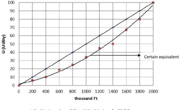
3. Then we draw a coordinate system. The X-axis is the range of interpretation, the Y- axis values in the utility. (Diagram 2)

to 1,000,000 Ft (a) 100 to 0 Ft (0) 0 Sign: U(a)Ft = 100; U(0)Ft = 0

Diagram 2: A graphical representation of utility equivalence

Based on this example the decision-maker‟s maximum utility value is 100 and this belongs to the 2,000 thousand. Marking:

U (2000 thousand) = 100, U (0) = 0

4. Then we determine the utility values between the two extremes. In each step, we quantify the utility values based on the well-known utility values using the following assumptions:

U (zFt) = 0.5 x U (xFt) + 0.5 x U (yFt) The first questions to be asked marked by questions K1:

K1 [0 HUF, the HUF] ~ b, which is 0 HUF, 2,000 thousand HUF] b ~ HUF

We accept that b = 1,300 thousand HUF. In this case, the utility of 1,300 thousand HUF can be calculated by the following formula.

U(b)Ft = 0,5 U(0Ft)+0,5xU(2,000 thousand HUF), U(b)Ft = 0,5x0+0,5x100

U(b)Ft) =50

This algorithm allows defining more utilitarian values. Their definition is always based on the well-known two adjacent utility values. (See Diagram 3 and Table 7 and for loss Diagram 4) Easy to see from the diagram that the decision-maker‟s risk-taking appetite by the utility function is well characterized. The ramp, the risk making is considered risk preference because large amounts are for increasing utility values .

Certain equivalent egyenérték

This function allows them with its help to determine the utility of the results instead of express the results in monetary terms. This utilitarian values - which well-expressed the preferences of the decision maker - are replaced in the proposed results of the decision matrix and quantify the expected utility instead of the expected value. Quantifying the utility values can be done

- by graphical method (see Diagram 2) and - function calculation.

For the calculation of the function, knowing the utility values, we determine the utility function by regression analysis. Then, the utility values can be calculated using the function.

(The function is substituted with the results.)

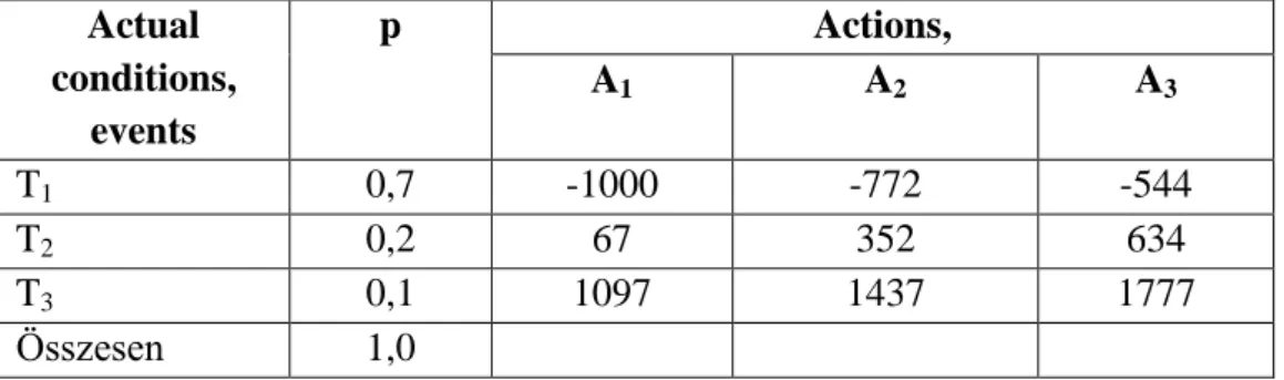
The calculation process: the utility function is substituted by the intended result. Performing the calculations, the utility of the planned result, the utility value is given. The utility value is corrected by the random coefficient and we obtain the expected utility. Assume the data in decision-making matrix:

Actual conditions,

events

p Actions,

A1 A2 A3

T1 0,7 -1000 -772 -544

T2 0,2 67 352 634

T3 0,1 1097 1437 1777

Összesen 1,0

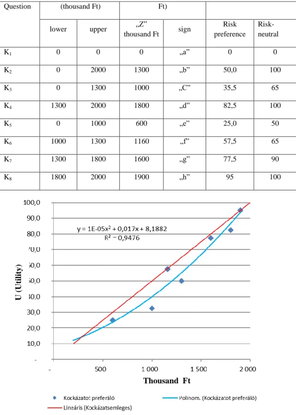
Table 7: The development of utility values

(What certain amount would the decision-maker, who prefer risk, replace in the following amount which is being obtained by 50-50% chance?)

Interval Biz. equivalent (thousand U (Utility)

Question (thousand Ft) Ft)

lower upper „Z”

thousand Ft sign Risk preference

Risk- neutral

K1 0 0 0 „a” 0 0

K₂ 0 2000 1300 „b” 50,0 100

K₃ 0 1300 1000 „C” 35,5 65

K₄ 1300 2000 1800 „d” 82,5 100

K₅ 0 1000 600 „e” 25,0 50

K6 1000 1300 1160 „f” 57,5 65

K₇ 1300 1800 1600 „g” 77,5 90

K₈ 1800 2000 1900 „h” 95 100

Diagram 3: The risk-taking decision maker’s utility function (Table 7)

thousand Ft

U (Utility)

Thousand Ft

Diagram 4: The risk-taking decision maker’s utility function in the situation of losses Knowing the utility functions the values in decision matrix can be calculated. The decision- maker’s utility function (Diagram 4):

U(x) = 1E-05x² + 0,017x +8,182 R² = 0,9954 Make the calculations:

U₍₆₃₄₎= 8,182 +0,017 * 634 + 0,00001* 634² U₍₆₃₄₎ = 22,96

The expected utility:

VU= 22,96*0,2 = 4,59 So that

Actual condi-

tions p

110 Actions, options for action (million Ft)

A1 A2 A3

E U VU E U VU E U VU

E1^* 0,7 -1000 -35,18 -24,62 -772 -27,26 -19,08 -544 -20,43 -14,30

E2 0,2 67 9,35 1,87 352 15,39 3,07 634 22,96 4,59

E3 0,1 1097 38,86 3,89 1437 53,2 5,32 1777 69,97 6,99

Total 1,0 -18,86 -10,69 -2,72

 The applied function U(x)= -1E-05x² + 0,017x -8,182

By applying the procedure: it allows taking into account the decision maker‟s preferences, calculating the outcome by taking into account the individual preferences can be consistent, the decision-maker is "in the absence" the decisions may be characteristic choices.

1.6. Application of the method KIPA

U (Utility)

As in the previous chapters KIPA method is presented essentially through an example to show the possible reasons for its applying.

TASK (Reset)

We accept the following. A group of investors - based on the assessed market situation – is trying to found a forage mixing plant. An important issue is for them the selection of the plant site. At the same time they wish to take into account several factors: potential buyers scope, accessibility (road network condition, distances), the size of local taxes, the presence of skilled labor. To judge the importance of each criterion they ask four experts to assist them.

They use the KIPA decision support method. This method contributes significantly to the professional merits of the decision and facilitates the decision-making. The final decision will be taken in accordance with a predetermined evaluation mechanism, thus avoiding excessive subjectivity influencing decision-making.

The KIPA model implemented on the basis of each pairwise comparison of the evaluation factors. Taking into account those properties in which one alternative is better than the other (preference) or investigate the worst properties of the preferable alternative as well (disqualifying). As a result, the decision is not only taking into account the improved properties but the worst properties were also tested, so if needed we can change our decision is based on the latter. The KIPA method has the distinction among the factors to be considered in the decision, weighting them. The decision alternatives are evaluated at first in essay, and then by scale transformation numerically. The decision will be based on the level of decision-maker‟s needs.

In the KIPA method, our decision is supported by the value of two indicators. Calculate the preference and the disqualification. In a pairwise comparison of decision alternatives each pair is determined by a value of both indicators. Each pair pointer determined by both a value in the pairwise comparison of decision alternatives. Consider the following simplified example to the understanding of the essence of two indicators: Assume that the selection of the site we only examine the amount of local taxes and accessibility. The amount of local taxes is more important decision-making factors such as accessibility. Possible alternative location for the site is a centrally located small city or small town. The small town has no local taxes, but the accessibility is very poor. The preference index shows favorable result for the local tax, since the small town is better in the very important decision factors. However the disqualification points out that while taking into account the importance of the deciding factors we can decide to the small town, there is a less important but still deciding factor (the accessibility) that it can be considered to refuse this alternative.

Let us return to the site selection problem of the investor group. The KIPA process of decision-support methods, has the following steps:

1. The evaluation criteria.

2. Weighting of the evaluation criteria.

3. Written evaluation (text-rating).

4. Text-Rating Scale Transformation.

5. Calculating preference and disqualification levels.

6. Determine the demand of own level.

7. Preparation of KIPA matrix and making the decision.

1. Creating the evaluation criteria: formulating questions for which answers need to look in the evaluation process. (The individual evaluation criterion is signed by Ei, where the "i"

means the i-th evaluation criterion.) Bases in the selected examples, the evaluation criteria are as follows:

E1: The scope of potential buyers E2: Accessibility

E3: Local Taxes size

E4: The presence of skilled labor

2. Weighting of the evaluation criteria: determination of the importance of the factors set out in the first point by using weights. To perform these task experts can call for help. Each expert will decide that which evaluation criteria are the most important. They give their responses in preference-table, where they examine that the terms of the first vertical column can be more important aspect than the term of the header. Where it is more important, they write 1 there.

The relative importance of the aspects to themselves is not interpreted, so in the matrix E1- E1, E2 - E2, etc. cells "X" is written. The summary of each expert‟s preference-tables is the aggregate preference-table from which the weight of the tested questions has been determined.

Four experts were invited. The preferences of the experts are shown in Table 8. Let us examine the first expert‟s preference-table: it is clear that it does not satisfy the principle of transitivity, as if E1 is more important than E2, E2 is more important than E3, than E3 can not be more important than E1. To avoid such cases, we use the consistency index (K), which examines the

“logical strength”, “reliability” of the experts' opinions. "K" value is added as a percentage.

Usually we stipulate in advance what will be accepted values.

Table 8: The appointed experts’ preference tables

1. EXPERT 2. EXPERT

E1 E2 E3 E4 E1 E2 E3 E4

E1 X 1 1 E1 X 1 1 1

E2 X 1 1 E2 X 1 1

E3 1 X 1 E3 X 1

E4 X E4 X

E1 is more important than E2 and E4 E2 is more important than E3 and E4 E3 is more important than E1 and E4

E1 is more important than E2, E3 and E4 E2 is more important than E3 and E4

E3 is more important than E4

3. EXPERT 4. EXPERT

E1 E2 E3 E4 E1 E2 E3 E4

E1 X 1 1 1 E1 X 1 1

E2 X 1 1 E2 X 1 1

E3 X 1 E3 1 X

E4 X E4 1 X

Opinion matches of the second expert

E1 is more important than E2 and E3, E2 is more important than E3 and E4,

E3 is more important than E1, E4 is more important than E2)

The consistency index is calculated using the following formula occurs:

where K = the consistency index

d = the number of inconsistent circle triplets

(d value can not be negative!) n = the number of evaluation criteria

a = shows you how many evaluation criteria were selected by the experts in the relevant valuation point of view (the sum of the numbers in the preference matrix rows)

Based on the foregoing, the expert opinion is taken into account only if K > 60%.

(Since the four evaluation aspects are at this issue (E1, E2, E3, E4) → n = 4.

2 - 12

) 1 2 )(

1

( ^{ }  ²

 n n n a

d

24

1 3

n n K d

 



Expert 1 Experts 2 and 3

E1 E2 E3 E4 a_i a_i² E1 E2 E3 E4 a_i a_i²

E1 x 1 1 2 4 E1 x 1 1 1 3 9

E2 x 1 1 2 4 E2 x 1 1 2 4

E3 1 x 1 2 4 E3 x 1 1 1

K1 = 60 % → accepted. K2 = 100 % → accepted.

Expert 4

E1 E2 E3 E4 ai ai2

E1 x 1 1 2 4

E2 x 1 1 2 4

E3 1 x 1 1

E4 1 x 1 1

∑a² = 10

K₄ = 20 % → do not accepted.

Because of the Expert 3‟s opinion is the same as the second expert, it is obvious that their preference-tables are to be the same, therefore the consistency indicators are to be the same.

We accept only experts 1, 2 and 3 opinions as in their cases the K > 60%.

Note that if in the preference-table above or below the diagonals with "X" marked only 1 is provided, the reviews are consistent, so the consistency index value is 100%.

Then we prepare the aggregate preference-table summarizing the opinion of experts, who are considered in the assessment.

The aggregate preference-table:

Experts 1, 2 and 3

1 2 12 - 12

) 1 4

* 2 )(

1 4 ( 4

1   



d 0

2 14 - 12

) 1 4

* 2 )(

1 4 ( 4

2   

d 

0,6 4 4

1

* 1 24

1 3 

 



K 1

3 3

0

* 1 24

2 3 

 

 K

2 2 10 - 12

) 1 4

* 2 )(

1 4 ( 4

4   

 d

0,2 4 4

2

* 1 24

4 3 

 

 K

Make up the aggregate preference table with columns which are necessary to determine the weights. (The examination of the assessors‟ and experts‟ agreement will be omitted, since the χ2-test beyond the material discussed in this note.) In the following we live with the assumption that the opinion makers‟ agreement is not accidental, but a consequence of their agreement.

The value of "a" have already been described above, the numbers in the rows is obtained as the sum of them

pa = preference ratio

k = the number of the considered experts

The example is based on the fact that k = 3, as three out of the 4 experts‟ opinion that we consider.

In case of E1: In case of E2:

In case of E3: In case of E4:

From the preference

E1 E2 E3 E4

E1 x 3 2 3

E2 x 3 3

E3 1 x 2

E4 x

E1 E2 E3 E4 ^ai p_a u z T

E1 x 3 2 3 8 0,792

E2 x 3 3 6 0,625

E3 1 x 2 3 0,375

E4 x 0 0,125

E1 E2 E3 E4 ^{ai pa u z T}

E1 x 3 2 3 8 0,792 0,81

E2 x 3 3 6 0,625 0,32

E3 1 x 2 3 0,375 -0,32

E4 x 0 0,125 -1,15

2 kn a k

p

i

a





0,792 4

* 3

2 3 8





a 

p 0,625

4

* 3

2 6 3





a  p

0,375 4

* 3

2 3 3





a 

p 0,125

4

* 3

2 3 0





a  p

ratio can be deduced for the "u" values:

u = „Pa” value assigned to standard random variable

(Appendix 1 contains the annex with the table of the standard normal distribution function of the random variable values.)

In case of E1: p_a = 0,792 → u = 0,81

First of all from the values in the table we choose the closest match to 0,792 and then from the vertical axis we assigned the "z" value to it (corresponding to the integers and decimal), and we supplement it with the value on the horizontal axis (corresponding to century).

In case of E2: pa = 0,625 → u = 0,32

In case of E3: p_a = 0,375 → u = - 0,32

As in the table of the standard normal random variable distribution function the minimum value is 0.5, so value of 0,375 is not included. By using the Φ (-z) = 1 - Φ (z) statistical correlation: 1-0.375 = 0.625 → 0.32 → -0.32 value is obtained.

In case of E4: p_a = 0,125 → u = - 1,15

Similarly, using the Φ (-z) = 1 - Φ (z) statistical correlation: 1-0.125 = 0.875 → 1.15 → -1.15 value is obtained.

Subsequently we transform "u" values to % to provide "z" option.

z = "u" value transformation to the scale of 0-100 (in %) as follows:

where: umin = the minimal „u” value umax = the maximum „u” value

u_i = the “u”' value (in the "i" line) to „E_i”

di = distance between „umin” and „ui” dmax = distance between „umin”és „umax” In our example:

Obviously, the minimum "u" value corresponds to 0% (E4), the maximum "u" value to 100%

(E1). The calculation of the values between them is as follows:

E1 E2 E3 E4 ^ai p_a u z T

E1 x 3 2 3 8 0,792 0,81 100

E2 x 3 3 6 0,625 0,32 75

E3 1 x 2 3 0,375 -0,32 42

E4 x 0 0,125 -1,15 0

dmax

z_i  dⁱ

umin ui umax

dmax

di

dmax = 1,15+0,81 = 1,96

dE2= 1,47

umin = -1,15 → 0% uE2= 0,32 umax = 0,81 → 100 %

% 75 0,75 96 , 1

47 , 1

2   

zE

Finally, we come to determine the actual weights. You need to decide how many pointed scale is used. We accept that a 5-pointed scale is used.

T = "z" is the value transformation to the weighting scale. Using scaling from 1 to 5 (z_max, 100 is divided into Tmax-1 parts, so that the zmin → Tmin and zmax → Tmax compliance is maintained). Accordingly, due

T zT

1 0

2 25

3 50

4 75

5 100

z₁=100 → 5, z₂=75 → 4, z₄=0→1 assignment does not cause any problem. Examine the case z3 = 42! Then zi is the value on "T" scale between 2 and 3, so 2 and a fraction will be the scale value. The fractional part calculation may be obtained by a simple ratio as follows:

(zi – zT)/zL, so (42-25)/25 = 0.7 therefore „T” = 2.7 This is rounded to 3, which is the actual weighting.

Content nominations in this context:

zi = the tested "z" value

z_T = the "z" value in the above table which is the closest to „z_i” from the bottom

zL = the scale of the table

The weights which are taken into account of the decision as aspects, are as follows:

E1: Potential buyers range (weighting is 5) E2: Accessibility (weighting is 4)

E3: Local Taxes size (weighting is 3)

E4: The presence of skilled labor (weighting is 1)

E1 E2 E3 E4 ^ai p_a u z T

E1 x 3 2 3 8 0,792 0,81 100 5

E2 x 3 3 6 0,625 0,32 75 4

E3 1 x 2 3 0,375 -0,32 42 3

E4 x 0 0,125 -1,15 0 1

% 42 0,42 96 , 1

83 , 0

3   

zE

dE2= 0,83

umin = -1,15 → 0% uE3= -0,32 umax = 0,81 → 100 %

dmax = 1,15+0,81 = 1,96