West - Hungarian University Faculty of Economics
István Széchenyi Management and Organisation Sciences Doctoral School
STATISTICAL TIME SERIES ANALYSIS AT STOCK
Doctoral (PhD) thesis
Polgárné, Mónika Hoschek
Sopron
2011.
Doctoral School: István Széchenyi Management and Organisation Sciences Doctoral School
Head of Doctoral School: Prof. Dr. Székely Csaba DSc
Program: Financial program
Head of Program: Dr. habil Báger Gusztáv CSc
Leader of research: Dr. Závoti József DSc.
………
Signature of Leader of research
Quote of the research, goals, and hypotheses
The author of the dissertation was inquiring into forecasting of time series during her study at the university. She was had her degree at finance so her thesis was a study of this two field of science. The goal of the thesis was to find a model good enough to characterize the evolution of the most important Hungarian stock index.
After university the author started to lecture statistics not to be too far from her field of research.
The aim of the writer was to characterize time series and build a proper model for develops of values of RAX, one of Hungarian stock indexes.
Hypotheses which were justified in dissertation:
H1: Statistical times series analysis if useful for characterize stock
H2: models made by newer methods are better to describe observed processes H3: One can make an even better model with a brand new mathematical solution.
Content, methods and justification of the research
Stock exchange is an organized institution, where transactions are under special rules, supervised, safe and transparent. Using continuous information investors rate securities and other listed products in every moment (Rotyis).
There are two methods of review of different money and finance market products:
1. Fundamental analysis: goal of the test is to define inner value. If the inner value is under the market price this means the good is overvalued. In this case there is high probability of price decrease of this instrument in order to approach the true value. If the inner value is over the market price, so the good is undervalued, the upward shift of price is expectable.
Fundamental analysis can help to recognize specifications of the concerned market, so one can make an established decision. Unfortunately it is not always enough. With the decision one can make a really successful transaction only if the market will behave as expected.
2. Technical analysis: They used to call chartists those who make technical analysis. The origin of this denomination is those chartists make and analyze charts to decide. There are two type of charts. One can make line chart and candlestick chart.
Every user can choose from the two chart type but must know that length of tested period can influence ideal choice. Candlestick chart carries a lot of important information if one examine only a short period. If the horizon is longer then a few month it can be technically hard to make chart, in this case should choose line chart.
Charts can help a lot even with drawing them but to make an efficient trading you need a bit more. That’s why they made indicators.
Toolbar of technical analysis contains lot of items which have statistical basis and which were used by author during her work.
The writer chooses RAX one of stock indexes which is the benchmark of investment funds.
She decided to use RAX because even Hungarian society reached a financial level where people have savings. If someone is not afraid of risks one can put savings to investment funds.
Because of diversification of gathered assets it is lower risk then a purely stock portfolio and that’s why chosen by many.
Rate RAX is officially published once a day at 16.30 since February 15, 1999. The basis of RAX was 1000 on January 7, 1998. The highest values until this day1 was 2146,21 almost three years ago in July 23, 2007.
During her research in Hungarian and international literature the author recognized that there are no single grouping for time forecasting, so her first job was creating an appropriate system. After unifying names of forecasting methods the next was making groups. Marking of books, notes, articles used for the dissertation were made to single form by the writer.
1July 31, 2010.
In history every procedure were refined and get perfected, just like it happened in statistical forecasting. The author used different forecasting methods of the most popular 70’s deterministic approach, and then she made forecasting by ARMA models from 80’s, and finally she used the youngest methods, ARCH models.
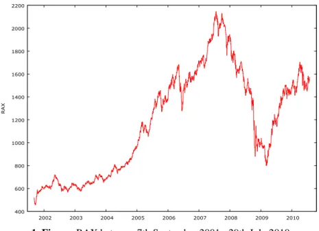
During research the writer used time series of RAX between 7th September 2001. - 29th July 2010. This means almost nine years and considers 2216 observation (1. Figure)
400 600 800 1000 1200 1400 1600 1800 2000 2200
2002 2003 2004 2005 2006 2007 2008 2009 2010
RAX
1. Figure: RAX between 7th September 2001.- 29th July 2010.
Decomposition models are using assumption that time series have four elements which can disconnected one by one and at the end of method there remain only the random element which has no effect to influence significantly time series value.
There can be two different relationships between elements of time series at decomposition models:
• Additive model: accumulating effects of times series elements
ij j ij ij
ij y c s
y = ˆ + + +ε (1.)
• Multiplicative model: multiplying effects of times series elements
ij j ij ij
ij y c S
y = ˆ ⋅ ⋅ ⋅ε (2.) where y value of time series
yˆ trend
c cyclical element s seasonal element ε random element
n
i=1,2,K, number of periods m
j =1,2,K, number of shorter periods in periods
During research the author build additive models.
The essence of first step of times series analysis is to filter other elements effects, to smooth time series. There are two methods to do this one is moving average and the other is analytical trend analysis.
If there is a hypothesis that durable trend can be approximate well with an analytical function, then the goal of trend analysis is to produce this function. To find the proper form of function is not a simple process. After one made a chart there can be more than one candidate for function form. The only way to find the best model which characterize investigated time series is to make all available models. There are three model selection criteria in use:
1. AIC – Akaike information criteria 2. HQ – Hannan-Quinn criteria 3. SIC - Schwarz information criteria
400 600 800 1000 1200 1400 1600 1800 2000 2200
2002 2003 2004 2005 2006 2007 2008 2009 2010
RAX
ötödfokú trend
fitted actual
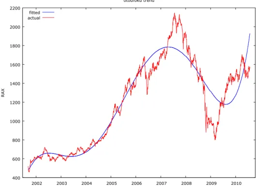
2. Figure: Time series of RAX and its polynomial trend degree of 5
2. Figure shows polynomial trend degree of 5, the best of examined analytical trends.
400 600 800 1000 1200 1400 1600 1800
2001 2002 2003 2004 2005 2006 2007 2008 2009 2010 2011
otodfoku_trend (original data) otodfoku_trend (smoothed)
-40 -20 0 20 40 60 80 100
2001 2002 2003 2004 2005 2006 2007 2008 2009 2010 2011
Cyclical component of otodfoku_trend
3. Figure: Cyclical element made by a polynomial trend degree of 5
There are two methods to define irregular medium- or long-term cyclical elements. One can get cyclical elements after compare against analytical and moving average trends. The difference between previously mentioned two methods is which trend was made before. 3.
Figure shows cyclical element of RAX time series.
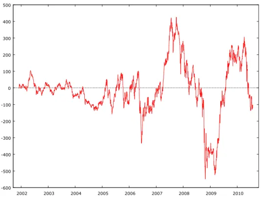
In order to define seasonality one has to filter out every other element’s effects. To do this one has to purify time series from effects of trend and cyclical element, i.e. subtract them form time series (4. Figure). One can make monthly or quarterly seasonality it depends on frequency of available data.
-600 -500 -400 -300 -200 -100 0 100 200 300 400 500
2002 2003 2004 2005 2006 2007 2008 2009 2010
4. Figure: RAX values only with random elements
Basic problem of trend analysis is to find a curve approximate well enough known values or (after depict them) points. In mathematics to solve this problem there are more solution, one is approximation.
There is a brand new method in mathematic which are able to combine good characteristics of regression and approximation as well. This procedure uses least square methods principle to choose weights and spline approximation is the result of iteration process (Polgár). The applied method with chosen weights is able to make robust estimation, which can used to filter out outliers or they can included with smaller weights.
At the first step of procedure one has to define number of splines ( N ) of curve. To down it one has to use available data to make an “experts” decision. The writer had chosen yearly, 200 daily, 50 daily stats so she made the trend form 9, 11 and 44 elements.
The second step of procedure is to decide what can be divide points (z0,z1,K,zN), where some curve-parts contact. One can chose from more than one option. First solution is where divide points are observed data, i.e. z0,z1,K,zN ∈
{
t1,K,tn}
. At the second solution intermediate points can get every value between observed data, i.e. z1,K,zN−1 ∈]
t1,K,tn[
, while define points at the ends of curve can be more options again. The solutions chosen by author the first observed data is the starting point of first spline and the last observed data is the end point of last spline, i.e. z0 =t1 és zN =tn.At the third step of procedure the minimum task is performed, where one has to get this correlation:
min )
) ( ( )
( 2
1 2 0
→
−
′′ +
∫ ∑
= i i
z z
N
i
i g z f
p
N g
λ . (3.)
The first element of this correlation is help the curvature values of classical interpolation/approximation spline, meanwhile the second element make robust estimation and lower the efforts of outliers.
1. Table: Errors of deterministic trends
Rising the number of subdivisions one can get better fitting trends. This can be shown confirmed with numbers in 1. Table, where there are sum of squares of errors and standard deviations of polynomial trend degree of 5 and different spline trends.
spline index
Polynomial trend degree of
5 N=9 N=11 N=44
SSE 55220330 13685822 9847620 4190320 Standard deviation 157,9286 78,62246 66,69248 43,50456
Among those who made analysis the most popular stochastic models were Box-Jenkins models for years. The two statistics whom method was named elaborated a three step method to define model parameters and to check goodness of prepared model.
Autoregressive moving average (ARMA model: )
q t q t
t t p t p t
t
t y y y
y =α1 −1 +α2 −2 +K+α − +ε −β1ε −1−β2ε −2 −K−β ε − (4.) In the process there are p autoregressive elements and q moving average elements, so the marking isARMA(p,q).
Tasks related to economical time series usually easily can be solved with ARMA models.
In the model made by the author there are only returns, not the real RAX values.
During ARMA model building a lot of time recovers a concept called stationary. If the expected value, the variance and the autocovariance2 of a random elements in a time series are not depend on time, then the time series are stationary. So
0 ) ( t =
E ε and var(εt)=σ2 and cov(εt,εt−k)=σ2⋅ρk where ρk the values of autocorrelation of experiment k .
The rundown of process is stable in time, there are no trend effects. Predictability of this type of time series is really high.
2 Autocovariance is independent from time, if given random element has no correlation with any previous random elements.
1. Identification:
In the first step of Box-Jenkins model one has to define parameters of ARMA(p,q) process, i.e. q and p parameters. The essence of this phase is to find theoretical time series which describe the best the empirical time series. During work it gives a big help if one make a chart form given data depend in time.
At this time get reveal what type of trend is in time series. If there can bee seen a linear trend, then if is enough to differential data set. Differentiation and thus filtering out trend is important because tested time series has to be stationary to estimate ARMA(p,q) process.
If data on chart seems to rise exponentially, then one has to make logarithm transformation on dataset first and then make a new chart.
To decide if there is a need of differential is another chart to draw beside of depicts investigated data in time. This called correlogram (autocorrelation function, ACF), which is a chart of autocorrelation coefficients, i.e. correlation coefficients of a dataset and its previous values.
) (
) , ( )
( ) , ) (
, ( )
( 2
t s t t t
s t t s
t
t E
E Var
Cor Cov s
r ε
ε ε ε
ε ε ε
ε − = − = −
= (5.)
On ACF chart r(s)is depending on s.
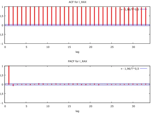
Drawing autocorrelation function (5. Figure) is helping not only to make time series stationary, but to give estimation for moving average (MA) elements q degree.
To determine autoregressive (AR) element p beginning value instead of correlogram one can use an other function called partial autocorrelation function (PACF). PACF purifies higher degree autocorrelation effects form lower degree autocorrelation effects.
-1 -0,5 0 0,5 1
0 5 10 15 20 25 30
lag ACF for l_RAX
+- 1,96/T^0,5
-1 -0,5 0 0,5 1
0 5 10 15 20 25 30
lag PACF for l_RAX
+- 1,96/T^0,5
5. Figure: RAX returns’ ACF and PACF functions
2. Estimation:
At this point of method the
q t q t
t t p t p t
t
t y y y
y =α1 −1 +α2 −2 +K+α − +ε −β1ε −1−β2ε −2 −K−β ε − (6.) equations parameters (hopefully) final values has to be estimated. The estimations are made by maximum likelihood (ML) method.
3. Diagnostically control:
At this phase one has to check if model fits data exactly, i.e. goodness of model. If described model is good, then random elements make a white noise process. To decide this Box and Pierce elaborated a test, where test statistic is
∑
=
= K
k
rk
n Q
1
2 (7.)
Its values have to be compared with a χK2−p−q distribution degree of freedomK −p−q.
Box-Pierce test has a serious problem. The test has a result which is not to reliable, that the reason why usually they make a second test called Ljung-Box test. The steps of the test are same as Box-Pierce tests, even hypothesizes and evaluations are the same, only test statistic value is computed otherwise:
∑
= ′−
′+
= ′
′ K
k k
k n n r
n Q
1 2
) 2
( (8.)
where n′=n−d, i.e. sample number minus number of differential.
If performed test show that built model is not efficient, then Box-Jenkins method has to restart with the first step. After modifying specification one has to make a new estimation and after test it. One has to continue method till test at third phase justify hypotheses, i.e. observed process is an ARMA(p,q) or ARIMA(q,d,p)process.
Great problem of ARMA models is stationary needed for them. However economy and especially stock time series random elements standard deviation in not constant in time. To solve this problem Robert F. Engle developed a new element of time series analysis stochastic family, called ARCH model.
) (q
ARCH model describable with three equations:
t m t t
t c y y
y = +φ − +L+φ − +ε
1 (9.)
t t
t ησ
ε = (10.)
2 2
2 2 2
1 1 0 2
q t q t
t
t =α +α ε − +α ε − + +α ε −
σ K (11.)
where ηt ~FAE(0,1) white noise.
First equation (8.) give observed variables expected value. One can see that variable is depending on its previous values, this means it is autoregressive element. If it is an AR(1) process, then it’s expected value is simplified to:
t t
t c y
y = +φ −1+ε (12.)
The value of deviation variable (εt) can get from second equation (9.). At this equation one can easily seen that random element is independent, however distribution is not equal distribution, its conditional variance changes in time.
Last equation (10.) due to previous random elements (innovation) effect. According to previous deviation is big enough then expected random element of given period is big too, while after small deviation comes small one. One can also see from equation that sign of deviation is not a matter because it disappears with cubic element.
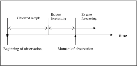
A properly built model is good not only to come to know better past, but to make forecasting by the help of it. During forecasting one applies already known regularities to determine forward in time observed phenomenon’s conformation, value. Forecasting has two types: ex post and ex ante (6. Figure).
6. Figure: Forecasting in time
During ex post forecasting not every available data get used to make the enquiry. Then from extend data not every one will be used in sample to prepare estimation but some get remained
time
Moment of observation Beginning of observation
Observed sample
Ex ante forecasting Ex post
forecasting
for checking. After preparation of ex post3 forecasting even those kept data help to make checking forecasting. The practical benefit of this type of forecasting is to rise to view how good the mounted model is. If forecasted and observed data substantially differ then one has to restart whole model building process.
Ex ante forecasting is good for time where no information is available. That’s the reason why here are no option to check model forecasting ability, one can only estimate it.
During forecasting one has to keep in mind that as time goes even a perfect model’s forecasting ability is rising too. Therefore is in way of doing forecast only for that much such as observed time was.
To process data and to build model author used an econometric program called GRETL (Gnu Regression, Econometrics and Time-series Library). Program approachable free of charge on internet4, or rather an old version of it is enclosed to one of two main econometric books distributed in Hungary. Trend made with splines get determined with the help of a program wrote in MapleV 5.
New research results
1. During her research author get known several grouping of time forecasting in literature.
This grouping was not covering each other. So during survey writer developed a uniform system which contains Hungarian and international grouping as well.
3 Ex post, i.e. reminiscent forecasting, but time forecasting is made this data are already known, they remain past.
4 http://gretl.sourceforge.net/
2. During research author used many method to analyze time series of RAX form 7th September 2001 to 29th July 2010. With leading approach till 70’s, i.e. deterministic time series analysis, a polynomial trend degree of 5 was the best to characterize observed data.
After detached trend with a moving average trend she was able to detect an almost seven years long cyclical element. Last filterable element was seasonality. Monthly and quarterly seasonality was calculated too. After these element only remain random elements which is not really interesting for deterministic time series analysis.
3. As degree of polynomial was raised during trend analysis so fitted the function even better and better. But raising degree at the same time worsens goodness of model. To eliminate this kind of problem author used a brand new type of spline to define trend. Thanks to this new mathematical solution she could better modeling basic tendency in time series then before with polynomials.
4. In the center of stochastic time series analysis is random element, which is not always random. Decrease of deterministic analysis was because of spreading autoregressive moving average (ARMA) models. After observing 2216 data author find time series not stationary.
After differential and with it filter out trend effect, she was able to fit an ARIMA (1,1,0) model, where first one refers to first degree autoregressive relationship between elements.
Second one refers to number of differentiations. Null means there are no moving average element is time series.
5. ARMA models are able to manage volatility, clustering of random elements. To solve this problem Engle developed ARCH (AutoRegressiv Conditional Heteroscedasticity) models, which were spread comprehensive in financial field, fight with great volatilities. For RAX’s nine years of time series author couldn’t fit a proper ARCH model, since rising of degree of autoregressive element model get better, so after a while estimation get too complicated, she had to choose an other method.
6. Bollerslev made generalization for ARCH models, which was named to GARCH (generalized ARCH) model. This could manage the problem of degree of autoregressive element. The writer started time series analysis with the simplest model AR(1)+GARCH(1,1), and at the end it came out the best by right of model selection criteria.
Suggestions
During deterministic time series analysis after filtering cyclical element and seasonality first degree of autocorrelation was detected between random elements by author in polynomials and even in spine trend too. In order to make a better usable model it would be necessary to determine the reason of this effect. Conceivable that it could be caused an effect well known in stock (e.g. calendar-effect, Easter-effect,…) and after taking to consideration autocorrelation could be eliminated.
The second field where are possibility to step ahead is ARCH models. Every survey gets a result that time series’ distribution is not a normal distribution. However there are members of ARCH model-family which are able to manage this problem. So later make these models to use building better models.
As a graduated economist it could be interesting for the author to analyze time series forecasting new method, she didn’t used so far. It is possible that already build models combining with econometric models results a much better model then previous.
Publications
Polgárné, Mónika Hoschek (2011): Forecasting in time. Szombathely: Határsávok II.
Polgárné, Mónika Hoschek (2010): Autoregression in time series analysis. Sopron: credit, World, Stage International Scientific Conference, ISBN:978-963-9883-73-4
Polgárné, Mónika Hoschek (2009): Comparison of forecasting methods. Kecskemét: EFTK II. 895.-899. o. ISBN 978-963-7294-75-4
Závoti, József - Polgárné, Mónika Hoschek – Bischof, Annamária (2009): Statistical compilation of formulas and tables. Sopron: NYME ISBN 978-963-9883-40-6
Polgárné, Mónika Hoschek (2005): Regression-analysis and using of it at economic practice.
Sopron
Polgárné, Mónika Hoschek (2005): Trend analysis, splines. Sopron: XXVII. OTDK, Phd section
Polgárné, Mónika Hoschek (2003): Stock analysis with mathematical-statistical methods.
Sopron, Conference of Hungarian Scientific Day
Polgárné, Mónika Hoschek (2003): Statistical methods at stock. Sopron
Polgárné, Mónika Hoschek (2001): Statistical methods used at Asamer - Horváth Ltd. Sopron, Pénzügyi szilánkok ISBN 963 00 7520 2
