Vol. 48(1) pp. 33–41 (2020) hjic.mk.uni-pannon.hu DOI: 10.33927/hjic-2020-06
IDENTIFICATION OF THE MATERIAL PROPERTIES OF AN 18650 LI-ION BATTERY FOR IMPROVING THE ELECTROCHEMICAL MODEL USED IN CELL TESTING
BENCE CSOMÓS∗1ANDDÉNESFODOR1
1Research Institute of Automotive Mechatronics and Automation, University of Pannonia, Egyetem u. 10, Veszprém, 8200, HUNGARY
The aim of this paper is to present an application of the generalized Warburg element and Constant Phase Element (CPE) for non-Fickian diffusion modeling. These distributed elements are intended to provide a better fit of low-frequency impedance data than the standard finite-length Warburg element in the case of most batteries. In addition, the current study demonstrates the ambiguity of the finite-length Warburg element if impedance data is insufficient within the very- low-frequency impedance spectrum. In order to select the appropriate Randles circuit for non-Fickian diffusion modeling, several configurations have been investigated. Based on the best fit of impedance data, the State-of-Charge (SoC) dependency of the Randles circuit parameters has also been analyzed. This study concerns a Samsung ICR18650-26F 2600mAh battery cell which was subjected to Electrochemical Impedance Spectroscopy (EIS) measurements between 10 mHz and 100 kHz as a function of SoC. The results were plotted and compared in the form of Nyquist plots. The Randles circuit parameters such as the resistancesRsandRct, double-layerCdl, leaky capacitance CPE and Warburg coefficients were estimated using ZView software. The present paper shows that CPE – and its QPE form – is a recommended choice to yield the best fit in terms of non-Fickian diffusion impedance. In addition, using CPE is a better alternative to avoid problems with initial values and multiple local solutions, which may exist in the case of the Warburg element. The resultant Randles circuit parameters and their SoC characteristics can be effectively used in further electrochemical modeling.
Keywords: Li-Ion Battery, Electrochemistry, Material, Battery model, Parameter estimation
1. Introduction
The State of Health (SoH) of a battery plays an important role in electric applications since it has a great influence on the available capacity and power of a battery [1]. SoH deteriorates with battery usage and the rate of aging is related to the operating history of the battery. Therefore, it is recommended to track the state variables of a cell throughout its life cycle and adapt the SoH prediction ac- cording to the current condition of the battery cell.
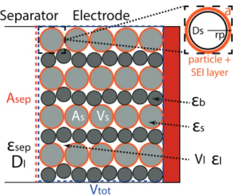
A common and reliable electrochemical model used in Finite Element Analysis (FEA) is based on the work of Newman et al. [2]. It consists of charge and mass balance equations in both solid (electrode) and liquid (electrolyte) materials, which describe the main operating character- istics of the cell. Even though these formulae could de- scribe the behavior of the cell in 3D, due to their high degree of nonlinearity and complexity, Pseudo-2D (P2D) modeling is favorable in terms of FEA [3]. It is also suf- ficiently representative to model wearout for automotive applications [4]. InFig. 1, a typical Pseudo-2D structure of a Li-Ion cell can be seen.
∗Correspondence:csomos.bence@gmail.com
Since battery manufacturing is still a developing sec- tor, the electrochemical composition of a cell constantly changes. Therefore, few battery-chemistry standards and complete databases can describe a given cell structure. In- sufficiently reliable and valid battery data inhibits battery modeling since a cell must always be inspected to de- termine its electrochemical parameters before modeling.
The standard way to obtain these electrochemical data is usually through an equivalent circuit modeling process with which the electrochemical properties of the cell can be extracted from EIS measurements.
2. Diffusion modeling techniques
It is possible to calculate battery-specific data using sev- eral techniques, which can basically be grouped into two types in terms of the measurement approach applied:
• direct measurements, which typically require disas- sembly of the cell, special preparations or an ex- perimental open-cell. These measurements can be, for example, different types of Electron Microscopy (EM), Computed Tomography (CT), titration, post- mortem analysis, etc.
rp
Electrode Separator
Asep
a
particle + SEI layer
Vs
As
ε
sD
lDs
ε
lε
sepε
bVl
Vtot
Figure 1:The relationship between the core material pa- rameters and components of the cell.Asep is addressed to the area of the separator.εsep, εb, εs, and εl denote the porosities of the separator, binder, solid matrix and void fraction, respectively.Dlrepresents the salt diffusion coefficient in the electrolyte.Dsstands for the diffusion coefficient in the solid electrode.Vl,VsandVtot are the volumes of the liquid, solid material and whole electrode, respectively.rpand a denote the average radius of each electrode particle and the specific surface area of the elec- trode.
• indirect measurements that do not require disassem- bly of the cell, e.g. current impulse excitation, Elec- trochemical Impedance Spectroscopy (EIS), gal- vanometry, potentiometry, chronoamperometry, etc.
[5]
EIS is a well-established and suitable method in the anal- ysis with regard to battery kinetics and has a solid back- ground in the literature [6]. Another advantage of EIS is that it does not require special preparation of the cell that would be extortionate and time-consuming.
Electrochemical parameters are formulated from EIS data in the form of resistive, capacitive, inductive or dis- tributed elements such as the Constant Phase Element (CPE) or Warburg element.
2.1 Standard equivalent circuits
In order to obtain battery-specific data, a Transmission- Line Model (TLM) was applied that is introduced and expounded on in [7]. It provides a generalized modeling solution for transport processes in porous electrodes by utilizing a finite number of serially connected resistor- capacitor (RC) pairs in parallel, which resolve the ion and electron transport appropriately. The network obtained in this way is considered to be ambiguous since various ar- rangements can be reduced to the same circuit resulting in identical resistance and capacitance of the circuit [8].
Although the number of RC pairs used can increase the resolution of the transport process and thus improve its accuracy, the increase in the number of elements results in stability as well as local and global optima problems due to equivocality. Since this is a major disadvantage of extended TLM networks, they are usually avoided.
W Rct
Rs C
dl
Figure 2:Randles equivalent circuit consisting of serial re- sistanceRs, charge-transfer resistanceRct, double-layer capacityCdland distributed impedance elementW.
A simplified form of TLM is the Randles equivalent circuit model (Fig. 2) which can be obtained if the the- oretical RC line of infinite length is reduced to a single Z-distributed element. In other words, the Z-distributed element models the limiting case of TLM. Its fundamen- tal principles and mathematical background are compre- hensively described in Barsoukov’s book [9]. The stan- dard Randles circuit model couples together the individ- ual characteristics of electrodes and electrolytes into one corresponding circuit element. The Randles circuit model consists of relaxation components such as the serial resis- tance of the electrolyteRs, charge transfer resistanceRct, a double-layer capacitorCdl and distributed impedance for modeling the low-frequency diffusive behavior of the cell. Usually, the double-layer effect exhibits non-ideal capacitive behavior so a CPE – the equivalent to a “leaky”
capacitor – should be used instead of aCdl. All of these detailed parameters of both electrodes are grouped to- gether, thus they represent the combined behavior of the two electrodes.
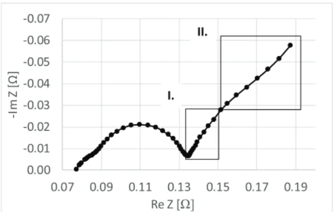
Ion transport that occurs in the low-frequency band- width of the impedance spectrum can involve diffusion, migration and convection, however, only diffusion is of interest because distributed elements are responsible for diffusion modeling. Diffusion modeling is the bottleneck of model development since it is related to a complex and interleaved electrochemical process that mainly charac- terizes the long-term operation of the battery. Ion trans- port can be, by and large, divided into two parts, namely lithium diffusion in the solid active electrode material and electrolyte. The “tail” at the beginning of the low- frequency bandwidth in the Nyquist plot shows diffusion in the electrolyte while the transition from the tail through an arc to a straightened end of the impedance curve de- picts the solid-phase diffusion inside the electrode matrix (Fig. 3). In fact, the cathode is composed of a poor ion- conducting material. A general rule of thumb is that its diffusion coefficient is2−4orders of magnitude smaller than the diffusion coefficient of lithium ions in the elec- trolyte, that is, the salt diffusion coefficient of the elec- trolyteDl falls within the range of10−10−10−11m2/s while the diffusion coefficient of lithium ionsDs in the solid matrix falls between10−13and10−14m2/s. In other words, the time constant for diffusion of Li-Ion transport is smaller in the electrolyte (∼ 10−100 s) than in the solid matrix (> 100 s). Consequently, the two types of diffusion need to be separated and should be modeled based on their different characteristic impedances.
-0.07 -0.06 -0.05 -0.04 -0.03 -0.02 -0.01 0.00
0.07 0.09 0.11 0.13 0.15 0.17 0.19
-Im Z [Ω]
Re Z [Ω]
I.
II.
Figure 3:A typical Nyquist plot of a Li-Ion cell; I. denotes a “tail” that mainly represents diffusion in the electrolyte;
II. shows a transition from liquid-phase to solid-phase dif- fusion.
Generally, diffusion is modeled by the classical War- burg impedance in accordance with the following as- sumptions: diffusion is Fickian (planar diffusion); the electrolyte is supporting, symmetric and binary; the cell remains in a quasi-equilibrium state during excitation;
and no reaction occurs in the bulk of the electrolyte. Un- der these premises, the standard Warburg impedance has an exponent of0.5 that implies its 45◦ phase angle. If diffusion occurs in an infinite reservoir where the con- centration can decrease to zero, infinite-length Warburg impedance can be assumed, otherwise diffusion is re- stricted and finite-length reflective or transmissive War- burg impedance can be assumed depending on whether the equivalent circuit is terminated by an open circuit or a resistor, respectively. The former and latter cases can be mathematically expressed by extending the standard infinite-length Warburg impedance with the hyperbolic functions tanh and coth, respectively. All three types of Warburg elements exhibit the same45◦ gradient at the beginning of the low-frequency bandwidth in the Nyquist plot.
In terms of impedance, using finite-length Warburg elements is unsuitable if an insufficient number of data points in the low-frequency bandwidth of the impedance spectrum are available to fit the hyperbolic functions well. This occurs when the EIS measurements typically run up until10mHz but some cells do not show a clear and distinct effect of diffusion in the solid phase. In this case, only the tail part of the impedance spectra can be reasonably modeled. Due to a lack of low-frequency data points, the finite-length Warburg elements cannot be ef- fectively applied. On the other hand, the tail part of the diffusion impedance can be modeled by CPE according to [11,12] which is a similar but more robust alternative to the Warburg elements.
All the transfer functions of the standard types of dis- tributed elements are summarized inTable 1. The transfer function of CPE can be expressed in two different forms according to the position of its time constant for diffusion
Table 1: Transfer functions of standard distributed ele- ments used in Fickian diffusion modeling [10].σdenotes the Warburg coefficient,ωrepresents the excitation fre- quency,τDstands for the diffusion time constant,Qis the QPE time constant,jdenotes the imaginary unit andRw
represents the Warburg resistance.
Name Impedance
infinite-length
Warburg Zilw(jω)= Rw
√jωτD
=σ 1
√ω(1−j)
finite-length
reflective Warburg Zflrw(ω)=Rwcoth(√ jωτD)
√jωτD
finite-length
transmissive Warburg Zfltw(ω)=Rwtanh(√ jωτD)
√jωτD
CPE ZCPE(ω)= 1
√jωτD
QPE ZQPE(ω)= 1
Q√ jω
τD. IfτDis emphasized from its square root, it is referred to as QPE, which sometimes provides a more stable re- gression than CPE.
Up to this point, only Fickian diffusion has been con- sidered that can be clearly identified by its square-root- like frequency dependency in terms of the transfer func- tion of the distributed elements. However, the impedance fit becomes more interesting when the cell impedance ex- hibits non-Fickian behavior, that is, the phase angle is not45◦due to diffusion non-idealities. These phenomena were investigated and are mostly related to multi-phase and multi-scale diffusion in porous electrodes [13,14], diffusion coupled with migration [15,16] and/or diffu- sion in non-conventional space [17–19]. Non-Fickian dif- fusion can be treated by fractional order circuits which consist of various types of typical configurations. In the literature [20], Warburg impedance is referred to as “gen- eralized” if it reflects the fractional intent. In this case, the Warburg exponent is generalized and denoted byγ, the dispersion parameter.
2.2 Equivalent circuit development for model- ing non-Fickian diffusion
In order to obtain the most accurate fit of the impedance curves, several configurations of the Randles circuit were developed. These setups are presented inFig. 4. The key differences between them can be explored in terms of both the position and type of the distributed elements in the circuit. In some papers from the literature, the dis- tributed element is in series withRct[21], while in others, it is placed in series with the parallelRct-CdlorRct-CPE branch. The distributed element can be either the War- burg element or CPE/QPE. Birkl et al. [22] shows that it is possible to model diffusion with an RC pair instead of a distributed element in the Randles circuit model. All of these configurations have been exhaustively expounded
Rs QPE
Rs W CPE
QPE
QPE Rct W
Cdl Rs
I.
II.
III. Rct Cdl Rs
W Rct Rs
CPE IV.
V.
Rct VI.
Rs
Figure 4:Different configurations of Randles circuits to study regression performance and fitness.W stands for Warburg element. The model of circuits I-IV, relaxation and diffusion are presented together while V-VI only focus on the tail part.
on in [23].
Based on these results, numerous Randles circuits have been evaluated to study the regression performance and fitness. InFig. 4, the arrangements of circuits I-IV model relaxation and diffusion simultaneously while V and VI only account for the tail part. The main reason for separation is that the stability and robustness of the impedance regression could be increased using this tech- nique.
The standard Warburg element and CPE/QPE had to be adjusted to match with the non-Fickian diffusion. At first, since only the tail part of the diffusion impedance was modeled, the hyperbolic part of the finite-length Warburg elements was neglected. Hence, the Warburg impedance was simplified to the infinite-length form.
Therefore, the Warburg impedanceZw had to be trans- formed into a generalized form by replacing the square root in the denominator withγ. As a result, the general- ized Warburg impedance could be written in the follow- ing form:
Zw(ω) = Rw
(jωτD)γ (1)
whereRwdenotes the Warburg resistance,ω stands for the excitation frequency,τDrepresents the diffusion time constant,j is the imaginary unit and0 ≤ γ ≤1. Now, thejγ term should be practically separated into real and imaginary components to reveal the contribution ofγto each part. Using Euler’s formula,Zwwas unbundled and grouped into real and imaginary parts:
Zw(ω) = Rw τDγωγ cos
π
2γ
− Rw τDγωγjsin
π
2γ
(2) τDused inEq. 2was then expressed as
τD=L1/γeff
Deff = β/γl,sepL1/γ0 βl,sepDl,0
(3) whereLeff denotes the effective diffusion length, Deff represents the effective diffusion coefficient,l,sepstands for the liquid fraction in the separator, and β is the Bruggeman coefficient. SinceτDis emphasized from the denominator ofEq. 1, the Warburg coefficientσcould be expressed as a fraction ofRwandτDaccording to
σ= Rw
τDγ . (4)
On the other hand, the transfer functions of CPE and QPE had to be transformed into
ZCPE(ω) = 1
(jωτD)γ (5) ZQPE(ω) = 1
τDγ(jω)γ (6) The updated transfer functions of the distributed elements enabled the non-Fickian diffusion to be properly fitted.
3. Experimental setup
This study is devoted to a commercial Samsung ICR 18650-26F cell with a nominal capacity of 2600 mAh.
It consists of a double-sided Nickel-Manganese-Cobalt (NMC) cathode and graphite anode according to the man- ufacturer’s datasheet.
The Samsung ICR 18650-26F cell was evaluated by EIS within the10mHz –100 kHz bandwidth at differ- ent States-of-Charge (SoC). The test was run at ambient temperature, namely25◦C, which was considered to be constant throughout. A Solartron SI1287 (Electrochemi- cal Interface) and a Schlumberger SI 1255 (HF Frequency Response Analyzer) were used for data acquisition. The Nyquist plot of the spectrum and the parametric fitting were produced by ZPlot and ZView software, respec- tively.
An auxiliary measurement had to be performed along with EIS to determine the cell’s Open Circuit Potential (OCP) characteristic at a 0.1 C-rated load current. The load current was generated by a TENMA 72-13210 Pro- grammable DC Load in Constant Current (CC) mode.
The data was recorded in NI PXI hardware that ran LabVIEW-based data acquisition software.
4. Analysis of the measurement results The purpose of the EIS analysis of the cell was to evalu- ate the fitness of the different Randles circuit models ac- cording to non-Fickian cell impedance data. On the other hand, the cell underwent another EIS measurement to detect how the parameters of the Randles circuit model changed during discharge. The EIS measurements pre- sented inFig. 5and6were made between10mHz and
-0.022
-0.017
-0.012
-0.007
0.08 0.09 0.10 0.11 0.12 0.13 0.14
Im Z [Ω]
Re Z [Ω]
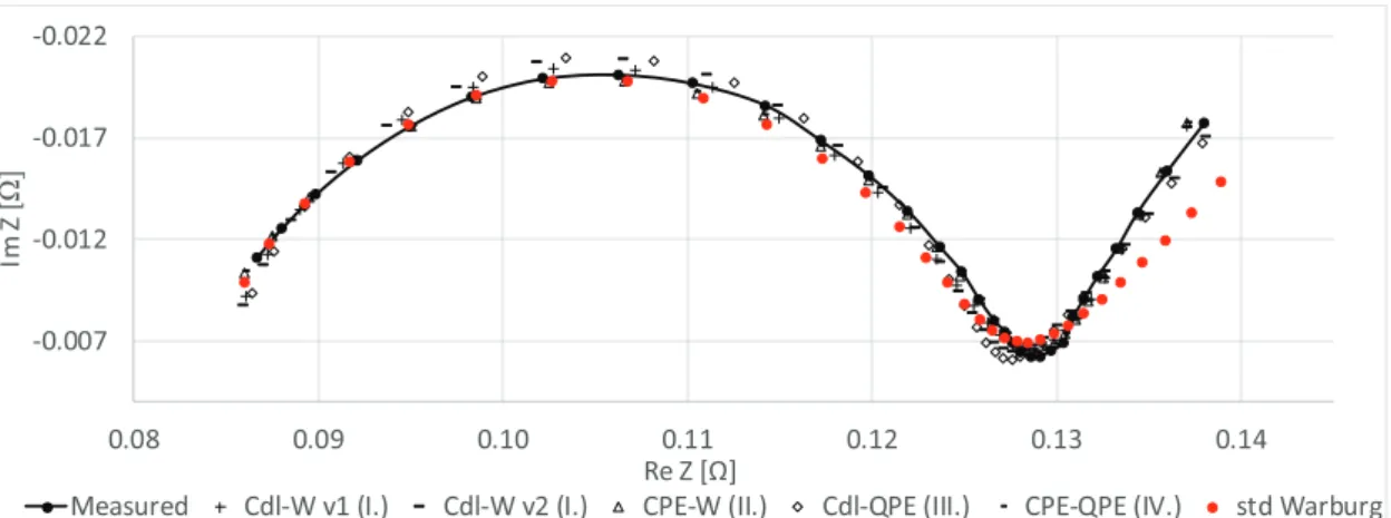
Measured Cdl-W v1 (I.) Cdl-W v2 (I.) CPE-W (II.) Cdl-QPE (III.) CPE-QPE (IV.) std Warburg Figure 5:Nyquist plot of the measured impedance and different fit functions (seen inFig. 4I-IV). v1 and v2 indicate that Warburg-based models were run on the basis of two different sets of initial parameters. The fit was performed between13Hz and10mHz at ambient temperature with a fully charged cell. The “std Warburg” was based on model I inFig. 4but with a Warburg exponent of0.5.
-0.018 -0.016 -0.014 -0.012 -0.010 -0.008 -0.006
0.118 0.120 0.122 0.124 0.126 0.128 0.130 0.132 0.134
Im Z [Ω]
Re Z [Ω]
Measured R-W R-QPE
Figure 6:Nyquist plot of the measured impedance and different fit functions (seen in models V-VI ofFig. 4. The fit was performed between80mHz and10mHz (only the tail part) at ambient temperature with a fully charged cell. The left part of the solid line is associated with the end of the relaxation semicircle and helps to locate the position of the tail.
13Hz where relaxation and diffusion occur. In the case of R-W and R-QPE pairs, only the tail part was mod- eled. InFig. 5, only a slight difference between the fits of the model is observed and the CPE-QPE pair shows the best match. Despite the insignificant difference between the non-Fickian models, a substantial improvement in ac- curacy can be observed especially with regard to fitting the tail when the standard Warburg element was replaced by any of the generalized Warburg- or CPE/QPE-based models.
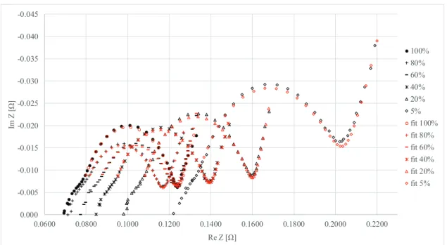
The changes in the Randles circuit parameters dur- ing discharge of the cell was also investigated further where only the best matching CPE-QPE pair was used for fitting. The resultant impedance plot is presented in Fig. 7. The EIS measurements were performed at20% SoC level increments. Every step of the discharge was followed by a12-hour-long period of relaxation before the EIS measurement was made in order to provide suf- ficient time for the cell to reach its stationary state. The impedance curves show that the degree of relaxation was high when the rate of the electrode reaction decreased or
if the transport of Li ions became limited. This occurred, for example, as the rate of Li diffusion decreased away from the interface. The evolution of changes in the dis- tinctive impedance curves could be tracked by changes in the parameters of the Randles circuits.Fig. 7shows that RsandRctsignificantly increased as SoC decreased due to the decreasing amount of Li-Ion particles engaged in the charge transfer process. Furthermore, the electrolyte resistanceRsincreased due to the decreasing ionic con- ductivity of the solution. All of these results agree with a well-known phenomenon, namely that the overall re- sistance of the cell increases during discharge. The shape and position of the plateau at the beginning of the semicir- cle was apparently due to a Solid Electrolyte Interphase (SEI) layer which formed on the anode particles that was unaffected during discharge. The presence of an SEI layer ascertains that the calendar and cycle lives of the cell both reduced. Since the gradient of the tails show significant similarities between100% and20% SoC, the diffusion time constant and diffusion coefficient of the electrolyte should change slightly during discharge. At5% SoC, the
-0.045 -0.040 -0.035 -0.030 -0.025 -0.020 -0.015 -0.010 -0.005 0.000
0.0600 0.0800 0.1000 0.1200 0.1400 0.1600 0.1800 0.2000 0.2200
Im Z [Ω]
Re Z [Ω]
100%
80%
60%
40%
20%
5%
fit 100%
fit 80%
fit 60%
fit 40%
fit 20%
fit 5%
Figure 7:Nyquist plots of the Samsung ICR 18650-26F2600mAh Li-Ion cell at different levels of SoC. The temperature was assumed to be constant at25◦C. The regression bandwidth was limited to between13Hz and10mHz. The small plateau at approximately250Hz is a consequence of a Solid Electrolyte Interphase (SEI) layer that formed on the anode particles. This shows that the calendar and cycle lives of the cell were reduced. The fit was made by the model of the CPE-QPE pair.
utilizable Li-Ions in the electrode became exhausted lead- ing to a significant decrease in both the rate of diffusion and reaction. On the other hand, the reaction rates did not vary extensively in the normal operating region since the
“valley” between the semicircle and tail possesses a sim- ilar imaginary component of the impedance.
In order to carry out cell characterization in the time domain, a quasi-equilibrium discharge was run using a 0.1 C-rated load current at a constant temperature of 25◦C. The OCV against SoC curve is presented inFig. 8 that exhibits typical discharge characteristics with a small plateau around 30% SoC and rapidly decreases below 10% SoC.
4.1 Determining Randles circuit parameters Evaluation of EIS data inFig. 5and the impedance re- gression were carried out by ZView software that applies
2.75 2.95 3.15 3.35 3.55 3.75 3.95 4.15
0 20 40 60 80 100
OCV [V]
SOC [%]
Figure 8:The Open Circuit Voltage (OCV) against State- of-Charge (SoC) characteristic of the cell.
the non-linear least squares method to fit and calculate the Randles circuit parameters. The results summarized inTable 2show that slight changes inRs,Rct andCdl
were observed with this setup. This was due to fitting on an almost ideal semicircle that exhibits a simple RC characteristic in the impedance spectrum. With regard to the estimation of diffusion time constants, diffusion in a real electrochemical battery cell is usually limited due to the relatively thin electrodes. Consequently, from a prac- tical point of view, ZView only has finite-length Warburg elements at its disposal. Since finite-length Warburg ele- ments should require data from the very low bandwidth that is unavailable in the present case, it is favorable to check the applicability of this type of element in the cur- rent case.
For this purpose, the Warburg parameters were esti- mated on the basis of two different sets of initial values as is denoted by v1 and v2 inFig. 5. Both cases yielded a similar fit but extremely different Warburg parameters.
Therefore, the estimation of Warburg parameters ran into multiple local solutions that erroneously characterize the same system with different diffusion time constants. This problem could be efficiently handled by using either the CPE+QPE pair or just QPE instead. The results are pre- sented inTable 3. Given theγwvalues, the Warburg ex- ponent is clearly far from0.5, hence the preliminary as- sumption of exhibiting non-Fickian diffusion was sub- stantiated. The maximum phase error between the stan- dard Warburg-element- and CPE+QPE pair-based Ran- dles circuit models was2.3% at10mHz. Since Randles circuit parameters are very sensitive due to the origin of their exponential functions, even a small improvement in
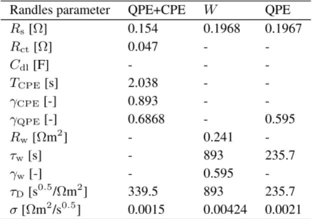
Table 2:The estimated Randles parameters where diffu- sion was only modeled by a Warburg element and a QPE in two different configurations. The QPE+CPE modeling technique was an effective way to avoid the uncertain- ties of finite-length Warburg elements due to a lack of data points in the very low bandwidth. The cell was fully charged and kept at25◦C.
Randles parameter QPE+CPE W QPE
Rs[Ω] 0.154 0.1968 0.1967
Rct[Ω] 0.047 - -
Cdl[F] - - -
TCPE[s] 2.038 - -
γCPE[-] 0.893 - -
γQPE[-] 0.6868 - 0.595
Rw[Ωm2] - 0.241 -
τw[s] - 893 235.7
γw[-] - 0.595 -
τD[s0.5/Ωm2] 339.5 893 235.7 σ[Ωm2/s0.5] 0.0015 0.00424 0.0021
fitting can significantly increase the accuracy in further electrochemical calculations based on these data.
The Randles circuit parameters were measured when the cell was fully charged but changed as the SoC level of the cell was altered as was seen inFig. 7. The estimated parameters at different SoC levels are summarized inTa- ble 4and their trends presented inFig. 9. The changes inRs andRct exhibited an exponential-like decreasing tendency against SoC whileRctslightly increased at ap- proximately100 % SoC. The increase inRswas due to the effect of a reduction in the ionic conductivity, while an increase inRctwas due to the decreasing rate of Li- Ion transfer through the electrode-electrolyte interface. In Fig. 10, the characteristics of changes in the CPE capacity and diffusion time constant can be seen. CPE slightly in- creased with discharge and its overall variance was about 0.4 F. This behavior along with the increase inRct can be attributed to the relaxation effect. Furthermore, less charge was available on the anode surface as the cell be- came fully discharged. The remarkable increase in diffu-
0 0.02 0.04 0.06 0.08 0.1 0.12 0.14
0% 20% 40% 60% 80% 100%
Resistance [Ω]
SOC level
Rs Rct
Figure 9: The trend ofRs andRct changes with SOC level. The cell shows a well-known increasing overall re- sistance during discharge.
Table 3:The estimated Randles parameters based on the configurations seen inFig. 4where diffusion and double- layer effect have been modeled by Warburg-element, QPE and CPE in different coupled configurations. In the table heading, W and C stand for Warburg and double-layer ca- pacitor, respectively. The cell has been at fully charged state and kept at25◦C.
Randles C+W C+W C+QPE CPE+W
parameter I II
Rs[Ω] 0.156 0.156 0.156 0.153
Rct[Ω] 0.041 0.041 0.041 0.047
Cdl[F] 1.731 1.731 1.73 -
TCPE[s] - - - 2.038
γ[-] - - 0.579 0.893
Rw[Ωm2] 0.0855 0.168 - 0.263
τw[s] 179 569.1 - 693.2
γw[-] 0.578 0.5792 - 0.687
τD[s0.5/Ωm2] 179 569.1 233.9 693.2 σ[Ωm2/s0.5] 0.0043 0.0043 0.0023 0.0029
sion time constants at approximately100% SoC implies that it was intended that diffusion coefficients should de- crease at the end of the discharge. This phenomenon plays a significant role in increasing the overall cell resis- tance especially when one of the electrodes is exhausted in Li.
5. Conclusions
The current work demonstrated an improved method of diffusion modeling. Several configurations of Randles circuits were studied in order to obtain the best fit of the impedance characteristics of a battery. The inappropri- ate fit of standard Warburg elements with regard to non- Fickian diffusion was corrected by applying generalized Warburg elements and CPEs. The proposed generalized model compensates well for the phase error between the measured and modeled impedances.
0 50 100 150 200 250 300 350 400
1.9 2.0 2.1 2.2 2.3 2.4 2.5 2.6
0% 20% 40% 60% 80% 100%
Diffusion time-constant [s]
CPE capacity [F]
SOC level
C_CPE tau_D
Figure 10:Charactersitics of changes in CPE capacity constants and diffusion time-constant. Diffusion time- constant remarkably increases during discharge that im- plies diffusion coefficients to decrease. The CPE does not change significantly.
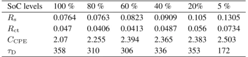
Table 4:The estimated Randles circuit parameters at given SoC levels based on the CPE-QPE Randles circuit model.
SoC levels 100 % 80 % 60 % 40 % 20% 5 %
Rs 0.0764 0.0763 0.0823 0.0909 0.105 0.1305
Rct 0.047 0.0406 0.0413 0.0487 0.056 0.0734
CCPE 2.07 2.255 2.394 2.365 2.383 2.503
τD 358 310 306 336 353 172
The finite-length Warburg element is a classical and generally applied tool in diffusion modeling, but it should be used carefully in some cases. The proposed work also shows that the finite-length Warburg element yields mul- tiple local solutions depending on its initial values if mea- sured impedance data is insufficient within the very low bandwidth of impedance. This leads to ambiguous results in terms of diffusion-related parameters which should be avoided, however, this problem can definitely be solved by applying CPE or QPE instead in diffusion models.
The Randles circuit parameters were estimated and can be used in further calculations to determine the elec- trochemical parameters of batteries [24].
Symbols
Binary diffusion coefficient of electrolyte Dl,0 m2/s
Warburg coefficient σ Ω/√
s
Diffusion time constant τD s
AC Excitation frequency ω Hz
Warburg exponent γ –
Electrolyte resistance Rs Ω
Charge transfer resistance Rct Ω
Warburg resistance Rw Ω
Double-layer capacitance Cdl F Acknowledgements
The research was supported by EFOP-3.6.2-16-2017- 00002 “Research of Autonomous Vehicle Systems re- lated to ZalaZone autonome proving ground”. We would like to thank Zoltán Lukács and Tamás Kristóf to support conducting EIS measurements in the laboratory of Fac- ulty of Physical Chemistry and sharing their knowledge in electrochemical modeling.
REFERENCES
[1] Redondo-Iglesias, E.; Venet, P.; Pelissier, S.: Effi- ciency Degradation Model of Lithium-Ion Batter- ies for Electric Vehicles,IEEE Transactions on In- dustry Applications, 2019, 55(2), 1932–1940 DOI:
10.1109/TIA.2018.2877166
[2] Doyle, M.; Fuller, T.F.; Newman, J.: 1-Modeling of Galvanostatic Charge and Discharge, J. Elec- trochem. Soc., 1993, 140(6), 1526–1533 DOI:
10.1149/1.2221597
[3] Mei, W.; Chen, H.; Sun, J.; Wang, Q.: The ef- fect of electrode design parameters on battery
performance and optimization of electrode thick- ness based on the electrochemical-thermal coupling model,Sustain. Energ. Fuels, 2019,3(1), 148–165
DOI: 10.1039/c8se00503f
[4] Lawder, M.T.; Northrop, P.W.; Subramanian, V.R.:
Model-based SEI layer growth and capacity fade analysis for EV and PHEV batteries and drive cy- cles,J. Electrochem. Soc., 2014,161(14), A2099–
A2108DOI: 10.1149/2.1161412jes
[5] Orazem, M. E.; Tribollet, B.: Electrochemical Impedance Spectroscopy,John Wiley & Sons Inc., 2008ISBN: 9781119363682
[6] Diard, J-P.; Gorrec, L.B.; Montella, C.: Handbook of Electrochemical Impedance Spectroscopy, 2017, 2–40http://www.bio-logic.info
[7] Falconi, A.: Electrochemical Li-Ion battery model- ing for electric vehicles. Material chemistry. Com- munaute Universite Grenoble Alpes, 2017, tel- 01676976
[8] Lasia, A.: Electrochemical Impedance Spec- troscopy and its Applications, Springer, 2014DOI:
10.1007/978-1-4614-8933-7
[9] Barsoukov, E.; Macdonald, J.R.: Impedance Spectroscopy, John Wiley & Sons, 2005 DOI:
10.1016/j.snb.2007.02.003
[10] Harrington, D.A.: Electrochemical Impedance Spectroscopy (thesis), 2004
[11] Huang, J.: Diffusion impedance of electroactive ma- terials, electrolytic solutions and porous electrodes:
Warburg impedance and beyond,Electrochim. Acta, 2018,281, 170–188DOI: 10.1016/j.electacta.2018.05.136
[12] Guha, A.; Patra, A.: Online Estimation of the Electrochemical Impedance Spectrum and Re- maining Useful Life of Lithium-Ion Batteries, IEEE Transactions on Instrumentation and Measurement, 2018, 67(8), 1836–1849 DOI:
10.1109/TIM.2018.2809138
[13] Huang, J.; Ge, H.; Li, Z.; Zhang, J.: An Agglom- erate Model for the Impedance of Secondary Par- ticle in Lithium-Ion Battery Electrode, J. Elec- trochem. Soc., 2014, 161(8), E3202–E3215 DOI:
10.1149/2.027408jes
[14] Huang, J.; Li, Z.; Zhang, J.; Song, S.; Lou, Z.;
Wu, N.: An Analytical Three-Scale Impedance Model for Porous Electrode with Agglomerates in Lithium-Ion Batteries,J. Electrochem. Soc., 2015, 162(4), A585–A595DOI: 10.1149/2.0241504jes
[15] Franceschetti, D.R.; Macdonald, J.R.: Diffusion of neutral and charged species under small-signal a.c.
conditions, J. Electroanal. Chem., 1979, 101(3), 307–316DOI: 10.1016/S0022-0728(79)80042-X
[16] Lelidis, I.; Ross Macdonald, J.; Barbero, G.:
Poisson-Nernst-Planck model with Chang-Jaffe, diffusion, and ohmic boundary conditions,J. Phys.
D: Appl. Phys., 2016,49(2), 25503DOI: 10.1088/0022- 3727/49/2/025503
[17] Sapoval, B.; Chazalviel, J.-N.; Peyrière, J.: Electri- cal response of fractal and porous interfaces,Phys.
Rev. A, 1988, 38(11), 5867–5887DOI: 10.1103/Phys- RevA.38.5867
[18] Jacobsen, T.; West, K.: Diffusion Impedance in Planar, Cylindrical and Spherical Symmetry, Electrochim. Acta, 1995, 40(2), 255–262 DOI:
10.1016/0013-4686(94)E0192-3
[19] Bisquert, J.; Garcia-Belmonte, G.; Bueno, P.;
Longo, E.; Bulhões, L.O.: Impedance of constant phase element (CPE)-blocked diffusion in film elec- trodes, J. Electroanal. Chem., 1998,452(2), 229–
234DOI: 10.1016/S0022-0728(98)00115-6
[20] Ramos-Barrado, J.R.; Galán Montenegro, P.; Cri-
ado Cambón, C.: A generalized Warburg impedance for a nonvanishing relaxation process, J. Chem.
Phys., 1996,105(7), 2813–2815DOI: 10.1063/1.472806
[21] Qu, D.: The study of the proton diffusion process in the porous MnO2 electrode, Elec- trochim. Acta, 2004, 49(4), 657–665 DOI:
10.1016/j.electacta.2003.08.030
[22] Birkl, C.R.; Howey, D.A.: Model identification and parameter estimation for LiFePO4 batteries, IET Conference Publications, 2013,2013(621 CP), 1–6
DOI: 10.1049/cp.2013.1889
[23] Zou, C.; Zhang, L.; Hu, X.; Wang, Z.; Wik, T.;
Pecht, M.: A review of fractional-order techniques applied to lithium-ion batteries, lead-acid batter- ies, and supercapacitors, J. Power Sources, 2018, 390(June), 286–296DOI: 10.1016/j.jpowsour.2018.04.033
[24] Nguyen, T.Q.; Breitkopf, C.: Determination of dif- fusion coefficients using impedance spectroscopy data, J. Electrochem. Soc., 2018, 165(14), E826–
E831DOI: 10.1149/2.1151814jes