CHAPTER TWELVE SOLUTIONS OF ELECTROLYTES

CHAPTER TWELVE

SOLUTIONS OF ELECTROLYTES

12-1 Introduction

The historical development of electrochemistry constitutes one of the more interesting stories of science. It begins, for us, with observations made in 1600 by W. Gilbert, physician to Queen Elizabeth, on the ability of amber to attract pith or other light objects when rubbed with a piece of fur. Gilbert coined the word electric (from the Greek for amber) in describing such behavior. Benjamin Franklin became interested in the subject and suggested, around 1750, that the different behavior of electrostatically charged glass and amber was not due to two kinds of electricity, but rather to an excess or deficiency of an electric "fluid." Thus began the subject of electrostatics, which culminated around 1890 with the identification of the electron as the unit of electricity.

Another chain of events led to the discovery of a second kind of electricity. The story traces back to 1678 when Swammerdam demonstrated before the Grand Duke of Tuscany that a frog's leg resting on a copper support would twitch when touched with a silver wire connected to the copper. We are more familiar with the experi­

ments of L. Galvani in 1790, who observed that a frog's leg (again) would twitch when connected to a static electricity generator or when the nerve was merely touched with a metal strip which was connected to the end of the leg. The terms galvanic electricity and galvanometer honor this discovery. By 1800 A. Volta succeeded in producing visible sparks from a stack of alternate silver and zinc plates. This was the first battery, then called a voltaic pile or a galvanic cell.

The first definite experiment in electrochemistry appears to have been made by W. Nicholson and A. Carlisle in 1800, who used a galvanic cell to electrolyze water. By 1807 H. Davy had isolated sodium and potassium by the electrolysis of their hydroxides.

The foundation of modern electrochemistry was laid by M. Faraday, working around 1830 at the Royal Institution. He showed that a given quantity of electricity produced a fixed amount of electrolysis and formulated the following now well- known laws:f

+ Faraday's law is not always experimentally obvious; for a puzzling discrepancy see Palit (1975).

429

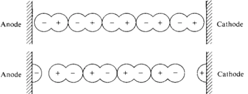
FIG. 1 2 - 1 . Illustration of the original Grotthus mechanism.

1. The amount of chemical decomposition produced by a current is propor­

tional to the quantity of electricity passed.

2. The amounts of different substances deposited or dissolved by a given quantity of electricity are proportional to their chemical equivalent weights.

Faraday's contribution is of an importance comparable to that of Joule in finding the mechanical equivalent of heat. In modern language, Faraday determined the electrochemical equivalence, or the amount of electricity corresponding to one mole of electrons. This equivalence, which we call the Faraday constant & is

= N0e = (6.02252 χ 102 3)(1.6021 χ 10~1 9) = 96,487 C mole"1, where 7V0 is Avogadro's number and e is the charge on the electron; C is the abbreviation for the coulomb. Our name for the natural unit of charge, the electron, was proposed, incidentally, by G. Stoney in 1874.

A great number of interesting and perceptive experiments have been passed over in this account. Much of our basic nomenclature originated during Faraday's time: anode and cathode for the positive and negative pole, respectively, of a battery; ion (Greek for wanderer) for the carrier of electricity in solution ; ampere for the unit of current; and ohm for the measure of electrical resistance. The latter two terms are, of course, in recognition of the pioneer investigations of A.M.

Ampère an d G.S . Ohm .

The mechanis m whereb y curren t i s transporte d throug h solution s o f salt s took nearl y a centur y t o b e understoo d afte r th e first observation s o f th e pheno - menon b y Dav y an d others . A n earl y ide a wa s tha t o f T . vo n Grotthus , wh o suggested i n 180 5 tha t a n electrolyt e consiste d o f pola r molecule s whic h line d u p in a n electri c field and , b y exchangin g ends , passe d electricit y dow n a chain . H e was tryin g t o explai n ho w electricit y coul d g o throug h a solutio n an d ye t caus e electrolysis onl y a t th e electrodes . A s illustrate d i n Fig . 12-1 , hi s though t wa s that applicatio n o f a potentia l acros s th e electrode s cause d th e pola r molecule s to brea k an d refor m i n suc h a wa y a s t o leav e a negativ e piec e o f on e a t th e anod e and a positiv e piec e o f anothe r a t th e cathode . Th e ide a wa s clever , an d wil l b e invoked i n mor e moder n languag e i n explanatio n o f th e motio n o f hydroge n ions . As originall y stated , th e Grotthu s mechanis m wa s untenabl e o n variou s grounds : Electrolyte "molecules " ar e no t tha t clos e togethe r i n solution ; wh y shoul d eve n the weakes t potentia l b e abl e t o caus e stron g molecule s t o brea k up ; an d s o on . The hypothesi s wa s largel y demolishe d i n 185 7 b y R . Clausius . Clausiu s propose d instead tha t th e positiv e an d negativ e part s o f th e electrolyt e molecul e wer e alway s partially presen t a s fragment s o r ions , whic h the n carrie d th e current . W e woul d

12-2 CONDUCTIVITY-EXPERIMENTAL DEFINITIONS AND PROCEDURES 431

call his proposal one of partial dissociation. It was a compromise in the sense that it was very difficult to accept that a molecule could break up or dissociate, and

Clausius theorized that only a small fraction of the molecules actually did so.

We come now to the last quarter of the nineteenth century. J. van't Hoff and his group made colligative property measurements on sugar solutions and then on aqueous electrolytes. They reported large / factors [Eq. (10-58)] in the latter case.

Thus / was close to two for NaCl solutions. S. Arrhenius drew heavily on van't Hoff's work in proposing the theory of electrolytic dissociation in 1883. The theory amounted to an assertion that electrolytes were mostly and not just partially dissociated into ions. During this last period the giants of electrochemistry were Arrhenius, F. Kohlrausch, W. Ostwald, and van't Hoff. Kohlrausch and his school carried out a monumental number of experiments on the conductance of electrolyte solutions, establishing that they obeyed Ohm's law. Thus the terms specific con­

ductivity and equivalent conductivity were defined, and the major rules governing the variation of conductance with concentration were formulated. Ostwald did much to clarify the behavior of what we now call weak electrolytes, or ones which behave essentially as Clausius had proposed much earlier.

The basic framework of electrochemistry was thus in place by the turn of the century. The early 1900's were spent in more and more precise studies of electrolyte solutions. The next major advances were made in the 1920's, in the treatment of the forces between ions, which determined the quantitative aspects of their motion through a solvent and their thermodynamic properties. A major theory by P. Debye and E. Huckel led, in 1923, to an enduring picture of dilute electrolyte solutions.

Each ion tends to have around it an excess concentration of oppositely charged ions, which form a statistical or diffuse atmosphere. This atmosphere contributes to the thermodynamic chemical potential of the ion and hence to its activity coefficient. At about the same time, J. Bronsted and N. Bjerrum (in Copenhagen) made lasting contributions both to the understanding of acid and base strengths and in establishing that ions could form ion pairs in more concentrated solutions.

Late in the same decade, L. Onsager extended the Debye-Huckel theory to treat dynamic effects such as conductance and diffusion. Later, with I. Prigogine, he was a leader in developing the general thermodynamic treatment of irreversible processes. Still later, R. Tolman and J. Kirkwood pioneered the development of the statistical mechanical theory of solutions—a task yet to be finished.

We begin the subject of electrochemistry with the important new property of electrolyte solutions—that of conductance. The separate behavior of each kind of ion is then discussed in terms of ionic mobilities and of transference numbers. The chapter moves on to a presentation of the Debye-Huckel treatment of the non- ideality of electrolyte solutions and concludes with a study of ionic equilibria.

12-2 Conductivity-

Experimental Definitions and Procedures

A. Defining Equations

The various systems of electrical units were reviewed in Section 3-CN-2. It was noted there that international commissions have recommended the uniform adoption of the SI system of units, one of the main advantages being that the esu

and emu systems are merged into a single one. Experimental electrochemistry makes use of the volt (V), ampere (A), coulomb (C), and ohm (Ω)—all accepted in the SI recommendations.

As noted in Section 3-CN-2, the ampere is defined in terms of the magnetic field produced by current / flowing in a loop of wire. The coulomb is the quantity of electricity q corresponding to a current of 1 A flowing for 1 sec, or in general, q = it (or J / dt). The unit of potential V is the volt; it requires 1 J (joule) of energy to transport 1 C of charge across 1 V potential difference. Resistance R is defined in terms of Ohm's law,

V = iR. (12-1) A current of 1 A flowing through a resistance of one ohm produces a voltage drop

of 1 V. The resistance R is, of course, a function of temperature and, in the case of electrolyte solutions, of concentration.

Ohm's law can be thought of both as an ideal law and as the limiting law for small V and /. It is well obeyed by all substances, provided the energy dissipated does not result in appreciable local heating. In the case of electrolyte solutions Ohm's law begins to fail at high voltages because ionic velocities become large enough that the distortion of the diffuse ion atmosphere around each ion ceases to be proportional to its velocity. In the case of metals current is carried by elec­

trons, and there is no problem in this last respect. The same is true for semicon­

ductors, which differ from metals mainly in that the concentration of conduction electrons is small and increases exponentially with temperature so that the resistance is very temperature-dependent.

The resistance of a substance is proportional to its thickness / and inversely proportional to the cross-sectional area si. One therefore generally reports a specific resistance or resistivity ρ defined by

R = ^P. (12-2)

The resistivity ρ is given in ohm centimeter in the cgs system and in ohm meter in the SI system. Although resistance is the measured quantity, its reciprocal, the conductance, is more useful in dealing with electrolyte solutions. Conductance L is defined as

L = \ (12-3) and specific conductivity κ as

p si R v J

As will be seen later, the ratio l/sf is usually treated as an apparatus or cell constant and is given the symbol k. Thus

R = kp, (12-5) κ = kL. (12-6) (A considerable range of symbols will be found for these quantities; the ones here

are the SI ones, except that L rather than G is used to denote conductance.) An electrolyte solution conducts electricity by several paths. Each ion contributes, including those from the self-ionization of the solvent. The situation is therefore

12-2 CONDUCTIVITY-EXPERIMENTAL DEFINITIONS AND PROCEDURES 433

one of resistances in parallel so that the total resistance obeys the law

- L = -L + -L + - L + . . . .

^ O b S ^ 1 ^ 2 ^ 3

Conductances are thus additive, that is,

A>bs =L±+L2+L9 + : . , (12-7)

hence their great utility in this situation. One is ordinarily interested just in the contribution to the observed conductance by the electrolyte and therefore subtracts out that due to the medium L0 :

L — Lobs — L0. (12-8)

The same relation will, of course, apply to specific conductivities:

κ = "obs — «ο · (12-9) One of the first quantitative observations was that the net specific conductivity

of a solution is approximately proportional to the electrolyte concentration. It should be exactly so if each ion were a completely independent agent since each would then make its separate, additive contribution to κ. A very useful quantity is therefore the equivalent conductivity, Λ, which is the value of κ contributed by 1 equiv of ions of either charge. We consider a portion of the electrolyte solution which is 1 cm deep and of area such that the volume contains one mole of charge due to the ions of the electrolyte (with only the positive or only the negative ions being considered). The number of moles of such charge per liter will be designated by C*, the concentration in equivalents of ions per liter whenever we wish to emphasize the distinction between actual ion concentration and equivalents of electrolyte per liter, C. The volume (in cubic centimeters) required to contain one mole of ions is 1000/C* and the area (in square centimeters) of the required portion of solution is then 1000/C*. It follows from Eq. (12-6) that

Λ (= L for 1 equiv) = — = κ —, k I or, since si = 1000/C* and / = 1,

Λ = ^ « . (12-10) The above language is somewhat carefully phrased. We want Λ to be the con­

ductivity ascribable to 1 equiv of actual ions. For a strong electrolyte, such as NaCl or N a2S 04 , C* = MN a Ci = 2 MNa2s o4 > and so on, where M is the molarity.

That is, C * is the molarity multiplied by the number of positive ion charges (or the number of negative ion charges) per formula weight, and corresponds to the usual definition of equivalents per liter. In the case of a weak electrolyte, such as acetic acid, however, C* should be the concentration of actual ions present per liter of solution; the concentration of undissociated acetic acid is not to be included.

If the solute is not fully dissociated or if there is doubt on the matter, one may write (12-11)

β . Measurement of Conductance

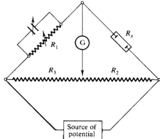
The actual quantity measured for an electrolyte solution is its electrical resistance R . This is usually done by means of a Wheatstone bridge, the basic scheme of which is shown in Fig. 12-2. In its simplest form, the galvanometer G shows no current flow when Rx/Ri = RJR3 · In practice, it is very important first of all that the electrodes of the cell used have identical electrode potentials; otherwise a voltage change across the cell will be present in addition to the voltage drop due to Ohm's law. This requirement is usually met by the use of identical reversible electrodes, such as platinized platinum, and an alternating source of potential. This last avoids having any appreciable net electrolysis at the electrodes and hence buildup of elec­

trolysis products. The use of the ac bridge introduces another problem, however, namely that due to the capacitance of the cell. There must now be a means for balancing out capacity differences across the two legs of the bridge, or otherwise the ac galvanometer (often an oscilloscope) will not register a point of zero current.

The reader is referred to experimental texts for further details.

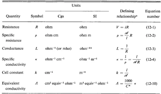
TABLE 12-1. Definitions of Electrical Quantities Units

Quantity Symbol Cgs SI

Defining relationship0

Equation number

Resistance R ohm ohm V = ÎR (12-1)

Specific resistance

Ρ ohm cm ohm m P = j R (12-2)

Conductance L o h m-1 (or mho) o h m- lb

R (12-3)

Specific conductivity

κ o h m-1 c m-1 o h m-1 m_1 ^{1 /}

~ ρ ~ ss/R (12-4)

Cell constant k c m-1 m -1

Equivalent Λ cm2 equiv-1 o h m-1 m2 equiv-1 o h m-1 A 1000 Λ = κ

c *

(12-10) conductivity

0 Here Κ is the potential difference and i the current between electrodes of effective area and separation /.

b The SI unit of conductance is called the Siemens, S, and has the dimensions A2 ^sec3 k g "1 ^{m ~}2^. where ΛΆΌΌ is the apparent equivalent conductivity, obtained with C, the formal concentration in equivalents per liter. " F o r m a l " means the number of gram equivalent weights of the solute present.

In the SI system, Eqs. (12-10) and (12-11) do not contain the factor of 1000.

Remember, however, that κ (SI) = 100/c (cgs) and that C and C* are now in equivalents per cubic meter, so that Λ (SI) = 10" M (cgs). If C is in moles m ~3, the SI designation for Λ is molar conductivity.

The various defining equations are summarized in Table 12-1.

12-2 CONDUCTIVITY-EXPERIMENTAL DEFINITIONS AND PROCEDURES 435

Source of potential

FIG. 12-2. Schematic diagram of a Wheatstone bridge.

The typical measurement, then, is of Rx, the resistance of the cell, first when filled with the solvent medium and then when filled with the electrolyte solution.

Application of Eq. (12-8) then gives the net conductance L due t o the solute.

The second experimental problem is the reduction of L to a specific conductivity κ. The defining equation (12-4) is not easily applied in practice since / is not exactly the distance between the electrodes and si is not exactly the area of the electrodes.

The reason is that ions lying outside of the cylinder defined by the two electrodes still experience potential gradients and contribute to the conductivity. Extensive and careful studies have allowed for this contribution, with the result that accurate specific conductivities are known for several standard electrolyte solutions. One such standard is a solution containing 0.74526 g KCI per 1000 g of solution, whose specific conductivity at 25°C is 0.0014088 o h m -1 cm-1. [See Daniels et al. (1956) for further details.] Alternatively, the specific conductivities of 0.1 M and 0.01 M KCI are 0.012886 and 0.0014114 o h m -1 c m -1 at 25°Q respectively.

The availability of precise, absolute specific conductivities allows the problem of determining the / and si values for a cell to be by-passed. One measures the resistance of the cell when filled with a standard solution and calculates the cell constant k by means of Eq. (12-5). The same cell constant applies to a measurement with any other solution (in very precise work, the standard and unknown solutions should have about the same resistance). One then uses k to calculate ρ or κ from the measured resistance R or conductance L.

Resistances can be measured with great precision, and conductance deter­

minations can therefore be extended to very dilute solutions. At this point, however, one must take major precautions to rinse the cell clean of any impurities adsorbed on the wall or on the electrodes and to free the solvent of all traces of electrolytes.

Kohlrausch and co-workers, for example, were able to obtain water virtually free of ionic impurities and found a residual specific conductivity of 6.0 χ 10~8 o h m-1 c m-1 at 25°C. As discussed in Section 12-4A this residual value is due to the ~ 1 0-7 mole l i t e r-1 of H+ and O H- ions from the dissociation of the water itself. This concen­

tration then represents the upper limit of dilution possible with an aqueous electro­

lyte before its contribution to the conductivity of the solution is swamped by that of the solvent water.

12-3 Results of Conductance Measurements

The decades preceding and following 1900 were ones in which the conductance of aqueous salt solutions was studied in great detail. Most soluble mineral salts, such as NaCl or K N 03, show a pattern of behavior which led Arrhenius to propose his theory of electrolytic dissociation, namely that salts are largely dissociated in aqueous solution and fully dissociated at extreme dilution. We agree with this interpretation today and call such substances strong electrolytes.

Other salts, and especially some acids and bases, behave quite differently from strong electrolytes. It is necessary to suppose that only a small degree of dissociation takes place; such substances are known as weak electrolytes. We take up these two categories of electrolytes in turn and then consider some of the more modern treatments of their behavior.

0 0.5 1 0 0.2 0.4 0.6

(c) (d) FIG. 12-3. (a) Specific conductivity is approximately proportional to C. (b) Equivalent con­

ductivity for strong electrolytes decreases with increasing C and (c) is nearly linear in Vc. (d) Equivalent conductivity decreases strongly with increasing C in the case of a weak electrolyte. All data are for 25° C.

12-3 RESULTS OF CONDUCTANCE MEASUREMENTS 437 T A B L E 1 2 - 2 . Some Equivalent Conductivities for Aqueous Electrolytes

at 25°Ca

Electrolyte

A b

(cm2 equiv-1 o h m- 1) Electrolyte

A b

(cm2 equiv-1 o h m- 1)

HC1 426.16 CaCl2 135.84

LiCl 115.03 Ca(N03)2 ^130.94

NaCl 126.45 BaCl2 139.98

KC1 149.86 N a2S 04 ^129.9

NH4C1 149.7 N a2C204 ¹²⁴

KBr 151.9 CuS04 ^133.6

N a N 03 ^{121.55 Z n S 0}4 ^132.8

KNO3 144.96 LaCl3 145.8

A g N 03 133.36 K4Fe(CN)6 ^184.5

NaOOCCH3 ^{91.0 NaOH 248.1}

MgCl2 ^129.40

a Source: H. S. Harned and Β. B. Owen, "The Physical Chemistry of Electro­

lyte Solutions," 3rd ed. Van Nostrand-Reinhold, Princeton, New Jersey, 1958.

b To convert to SI units, multiply by IO"4; thus A(HC1) = 426.6 x 1 0 ~4 m2

equiv"1 ohm"1.

A. Strong Electrolytes

It is typical of a strong electrolyte solution that its specific conductivity is propor­

tional to its concentration, to a first approximation. This behavior is illustrated in Fig. 12-3(a), and its observation led to the introduction of equivalent conductivity Λ as a useful quantity. According to Eq. (12-10), κ should be a linear function of concentration if Λ is an intrinsic property of the electrolyte, independent of its concentration. The linearity law is not exact, however; as shown in Fig. 12-3(b), Λ for typical strong electrolytes decreases noticeably with increasing concentration.

It was found very early that the decrease was proportional to V C ; that is,

Λ = Λ0 - A VC*, (12-12)

where, in the case of a strong electrolyte, we take C = C*. Figure 12-3(c) shows that Eq. (12-12) is well obeyed up to about 0.1 M uni-univalent electrolyte con­

centration. Deviations set in much earlier, however, with more highly charged ions.

As is discussed in more detail in the Commentary and Notes and Special Topics sections, Eq. (12-12) has been explained theoretically as a consequence of interionic attractions and repulsions, that is, as a result of long-range Coulomb forces between ions. The effect is, in a sense, an incidental one arising from the charge on ions rather than from more chemical properties. The most important specific charac­

teristic of an electrolyte is therefore Λ0, its équivalent conductivity at infinite dilution, since in this limit interionic attraction effects have vanished. Table 12-2 summarizes some Λ0 values for common electrolytes.

One of the early observations that helped to establish the concept of a strong electrolyte was that their Λ values are approximately additive. By this is meant that, for example, ΛΚ€ι is due to independent contributions from K+ and Cl~ ions, and similarly for ^Na N o3 and ΛΚΝ Ο3 . An example of additivity behavior would then be

^ N a C l — ^ K C l + ^ N a N O a ~ ^ K N 03 · (12-13)

Values at 25°C are

0.1 M 106.74 = 128.96 + 98.7 - 120.40 - 107.26, Λ0 126.45 = 149.86 + 121.55 - 144.96 - 126.45.

The first line of these data shows that the additivity rule holds to within a percent or so for 0.1 M solutions. Our interpretation of AQ requires that the rule hold exactly at infinite dilution, and this expectation is confirmed by the second line.

The additivity rule allows the indirect calculation of Λ for an electrolyte. F o r example,

^ A g C l — A \ g N Os + ^ K C l — ^ K N 03

= 133.36 + 149.86 - 144.96 = 138.26.

This type of calculation is greatly simplified in Section 12-6 since it turns out that absolute values for the individual ion contributions to Λ0 can be determined. One then obtains the value for an electrolyte by adding the separate ion values.

β . Weak Electrolytes

One of the early problems was that not all electrolytes behaved as illustrated in Fig. 12-3(a-c). Thus, unlike HC1 and N a O H , acetic acid and aqueous ammonia give the results shown in Fig. 12-3(d). In this case, however, the behavior was explainable on the basis of a dissociation equilibrium. For a binary electrolyte AB whose formal concentration is C we write

AB = A+ ^{+ B~ ,}

(1 — oî)C OiC OiC

where oc i s th e degre e o f dissociation . Th e equilibriu m constan t i s

* = ^ ^ = ^ ! £ - . (12-14 )

(1 — 0L)C 1 — oc

Alternatively, th e quotien t o f Eqs . (12-10 ) an d (12-11 ) give s

l a p p

Λ Γ*

Λ (12-15)

The ratio C*/C is that of the concentration of ions, aC = C*, to the formal concentration C, and hence is equal to a . Substitution of this result into Eq. (12-14) gives

Α2 Γ Λ(Λ - /lapp)

If interionic attraction effects (see Section 12-3C) can be neglected, as is often true for weak electrolyte solutions if their actual ionic concentrations are low, then Λ is identified with Λ0 ; Eqs. (12-15) and (12-16) then become

= α (12-17)

and

12-4 SOME SAMPLE CALCULATIONS 439 Equation (12-18) is known as the Oswald dilution law, after W. Ostwald, who proposed it. It allows a determination of the dissociation constant of a weak electro­

lyte from conductance data.

C. General Treatment of Electrolytes

The great success of Eq. ( 12-18) in accounting for the behavior of weak electrolytes such as acetic acid led Ostwald, Arrhenius, and others to apply the same equation to salts such as KC1 and to acids such as HC1. The results were confusing. Although the Κ values computed on the basis of Eq. (12-18) were reasonably constant for a weak electrolyte, they would vary 10- or 20-fold when so computed for strong electrolytes over a range of concentration.

It was eventually realized that two different effects are present. The predominant one in the case of a weak electrolyte is that of its partial dissociation into ions.

Superimposed on this, however, is the effect of interionic attraction, which causes the value of Λ (as distinct from ΛΆΏΡ) to vary with concentration. If the electrolyte is largely or fully dissociated, then the interionic attraction aspect becomes the dominant one. This is the situation with strong electrolytes.

Neither effect can be neglected for any electrolyte. In the case of a weak electro­

lyte the correct equation to use is Eq. (12-16), where Λ must have the value corre­

sponding to the actual ionic environment that is present. That is, the dissociation produces an ion concentration C*, which in turn affects Λ according to Eq. (12-12).

The constant A of this equation,

Λ = Λ 0- Α VC* [Eq. (12-12)],

has been evaluated theoretically (see Special Topics), and is given by

A = 0.2289Λ + 60.19. (12-19) Equation (12-19) is valid for aqueous univalent ions at 25°C at concentrations

below about 0.1 M.

12-4 Some Sample Calculations

A. Calculation of Dissociation Constants

The first two examples are ones in which interionic attraction effects are neglected.

That is, we assume that Λ0 gives the equivalent conductivity of the ions. We obtain the data in Table 12-3.

T A B L E 1 2 - 3 .

Measured resistance

Solution at 25°C (ohms)

Solvent water 1 x 10e

0.1 MKC1 24.96

0.01 M acetic acid 1982

We wish to calculate the dissociation constant of acetic acid. It is first necessary to obtain the cell constant. The net conductance due to the KC1 is

1 - = 0.04006.

24.96 106

The specific conductivity of 0.1 M KC1 is known to be 0.012886 o h m-1 c m- 1, and use of Eq. (12-6) gives the cell constant:

. κ 0.012886 1

Τ = "ÔÔ4ÔÔ6~ = ° ·3 2 17 α * -1· The net conductance of the acetic acid is

1 1 = 5.035 χ IO"4,

1982 106

from which we find

κ = (5.035 χ 10-4)(0.3217) - 1.620 χ 10~4. The apparent equivalent conductivity is therefore

ΛΕ ΡΡ = 1.620 χ 1 0 "4 = 16.20 c m2 e q u i v "1 o h m "1.

We may obtain Λ0 for the ions of acetic acid from the additivity rule, using the values 91.0, 426.2, and 126.5 for the Λ0 values of sodium acetate NaAc, HC1, and NaCl, respectively:

^ O . H A C — ^ O . N a A C + ^ O . H C l — A ) , N a C l

= 91.0 + 426.2 - 126.5 = 390.7.

The degree of dissociation is then 16.20

~~ 390.7 and the dissociation constant is

= 0.0415

(0.0415)*(0.01) - . 1 7 9 7 x l Q

K~ 1 - 0 . 0 4 1 5 x ιυ *

The resistance of 1 χ 106 quoted for the solvent water was deliberately picked as a somewhat low value. It corresponds to a specific conductivity of

K = (10-6)(0.3217) = 3.217 χ MO"7 o h m "1 cm"1.

The value for pure water was quoted in Section 12-2B as 6.0 χ 10~8 o h m-1 c m- 1, and the difference, 2.62 X 1 0 "7, is therefore to be attributed to impurities. Taking NaCl as a typical impurity, we get the corresponding concentration from Eq. (12-10) using A0 = 126:

C = I Ç M

rooo

Λ Izo

This concentration of ionic impurity is not likely to affect the dissociation of the

12-4 SOME SAMPLE CALCULATIONS 441

0.01 M acetic acid, so the slightly impure water used is acceptable for the particular experiment.

A value of 6.0 χ 1 0-8 o h m-1 c m-1 for the specific conductivity of pure water at 25°C was obtained by Kohlrausch and co-workers in 1894; the measurement allows a calculation of the dissociation constant for water itself. We write

H20 = H+ + OH-, Kw = (H+)(OH-). (12-20)

The concentration of water does not appear in Kw since we take pure liquid water to be the standard state for water substance, and hence of unit activity. The limiting equivalent conductivity for the electrolyte H+, O H- may again be calculated from the additivity rule:

Λ, Η + , Ο Η " = ^ 0 , H C 1 ^ 0 , N a O H ~ A),NaCl

= 426.16 + 248.1 - 126.45 = 547.81.

Equation (12-10) then gives the concentration of ions present:

C = (6· ° X "18) =0 1-10 Χ "17· 0 The value of Kw at 25°C is therefore

Kw = (1.10 χ 1 0 "7)2 = 1.20 χ 1 0 "1 4.

It is very difficult to remove the last traces of ionic impurities from water and this value for Kw is a little high; a better (modern) value is

Kw = 1 . 0 1 X 10~1 4. (12-21)

β . Correction for the Inter ionic Attraction Effect

We can improve the preceding calculation of the dissociation constant for acetic acid if we correct for the error introduced by using A0tUAc rather than AR + t A c- in determining it (we write ΛΗ+Α ο- as a reminder that this is the actual equivalent conductivity of the ions H+ and A c " ) . The value of 0.0415 for a is now regarded as a first approximation, giving an ion concentration

C * = (0.0415X0.01) = 4.15 χ 1 0 "4 M.

The constant A of Eq. ( 1 2 - 1 2 ) is as given by Eq. ( 1 2 - 1 9 ) , A - ( 0 . 2 2 8 9 X 3 9 0 . 7 ) + 6 0 . 1 9 = 1 4 9 . 6 2 .

Equation ( 1 2 - 1 2 ) then gives

Λ Η - , Α Ο - = 3 9 0 . 7 - ( 1 4 9 . 6 2 X 4 . 1 5 χ 1 0 "4)1 /2 = 3 8 7 . 7 .

The second approximation to α is therefore

C. Calculation of Solubility Products

A useful application of conductivity measurements is to the calculation of the solubility of slightly soluble salts. Consider the following set of data: The resistance of a cell is 227,000 ohms when filled with water and is 21,370 ohms when filled with saturated calcium oxalate solution. The cell constant is 0.25 c m- 1.

We calculate first the net specific conductivity of the calcium oxalate. The specific conductivity of the water is, by Eq. (12-4), 0.25/227,000 = 1.10 χ 10~6 (the water is again somewhat impure), and that of the saturated solution is 0.25/21,370 = 1.170 χ 10~5. The net value is 1.060 χ 10~5 o h m -1 cm"1. The value of A0 for C a2+ and oxalate, O x2 -, ions is obtained through use of the additivity rule:

^ o , C a2 +^{, O x}2^- = ^ 0 , C a ( N O= 3⁾2 ^ o , N a2O x ~ ^ 0 , N a N O3

= 130.94 + 124 - 121.55 - 133.

An equivalent conductivity for a salt such as C a ( N 03)2 will often be written as

^ L c a( N o3)2 as a reminder that 1 equiv and not one mole of salt is present in the defining experiment for A. We will take this point t o be implicit in the writing of a A value, and will insert such fractions only when the reminder seems desirable.

The concentration of C a2+ a n d O x2- ions is then

c = ,

w

*

'

The solubility product is, of course

CaOx(j) = Ca2^{+ + Ox}2^{~, K}sv ^{= ( C a}2 +^{) ( O x}2^{~ ) .}

The concentration of CaOx(s) does not appear in Ksp since solid calcium oxalate is in its standard state and hence has unit activity. The concentration is in equivalents per liter, so the molar concentration of ions in the saturated solution is 3.99 χ 1 0 -5 M. The value of Ksv is therefore (3.99 χ 10~5)2 = 1.59 χ 10~9 mole2 liter-2.

12-5 Ionic Mobilities

The conductance of an electrolyte solution is understood to be due to the motion of ions through the solution as a result of the applied potential. Positive ions move toward the electrode which is negatively charged in solution, or the cathode, and negative ions move toward the electrode which is positively charged in solution, or the anode. The current due to each ion is given by the product of the velocity of The change is small enough in this case that another round of approximation is not needed (but may be carried out by the reader as an exercise). The final value for Κ is now

g - T c S T -

* *

" - <

-

>

12-5 IONIC MOBILITIES 443

the ion and its charge. We consider first the quantitative aspect of this motion of ions under the influence of an applied potential, and then methods for measuring ion velocities.

A. Defining Equations

The motion of a particle in solution when subjected to some f o r c e / w a s discussed in Section 10-7A. To review the situation, we recall that a limiting velocity ν is quickly reached such that

v=£, '(12-23) where f is the friction coefficient. In the case of spherical particles, recall that a

relationship due to Stokes gives / = 6πψ, where η is the viscosity of the medium and r is the particle radius. It has become customary when dealing with ions to use the reciprocal of / , called the mobility ω. Equation (12-23) thus becomes

ν = œf. (12-24 )

We wan t no w t o conside r th e cas e o f a n io n i n solutio n whic h experience s a force du e t o th e impose d potentia l differenc e betwee n th e electrodes . Th e potentia l energy φ of a charge q in a potential V is, by the definition of potential, just qV (and will be in joules if q is in coulombs and V in volts). The force acting on a particle of this charge is then άφ/dx or q¥, where F is the field and is equal to dV/dx. The force in dynes is then

/ = WFze, (12-25) where F is in volts per centimeter, ζ is the valence number of the ion, and e is the

electronic charge in coulombs, e = ί.602 χ 1 0- 1 9C If the charge is given in esu, Eq. (12-25) becomes

/ = F z ^ . (12-26) The velocity of the ith ion is

υ,, = 107Fz«cu,e (12-27)

or

ν4 = K,F, (12-28)

where ut is called the electrochemical mobility, usually expressed as (cm s e c- 1^{) /} ( F c m- 1) or cm2 F-1 s e c- 1, and

Ui = 107ζ,ω<*. (12-29)

We now want to determine the equivalent conductivity of this ion. According to the definition of equivalent conductivity, the electrodes are to be 1 cm apart and of area such that the enclosed volume contains 1 equiv. The conductance so measured is then the equivalent conductivity. In the present case the current carried will be

U = v ^ , (12-30)

B. Measurement of Ionic Mobilities

The rate of motion of a given kind of ion under an imposed electric field may be observed directly if a boundary is present between two kinds of electrolytes. The method, called the moving boundary method, is illustrated schematically in Fig. 12-4.

A vertical tube is layered with a solution of M X ' (sodium acetate in this example) on top of one of M X (sodium chloride), which in turn is on top of one of M ' X (lithium chloride). The concentrations are such that the solutions decrease in density upward, so that convectional mixing will not occur. The applied potential is such as to cause positive and negative ions to move in the directions shown. The lower boundary is one between M ' X and MX, and hence between two types of positive ions, while the upper boundary is between M X and MX', or between two types of negative ions. The positions of these boundaries can be measured optically (and would also be visible to the eye) because of the change in refractive index.

A further requirement is that the mobility of M be greater than that of M ' and that the mobility of X be greater than that of X'. In terms of the particular example,

WNa+ > uLi+ and uci- > uAC-. If this condition is met, then M ' cations will not since Faraday's number gives the charge per equivalent. The potential difference is just F, since the electrodes are 1 cm apart, and we find from Ohm's law

1 ^{Ri F F F} or

λ, = u^. (12-31) It is customary to use the lower case lambda, λ, to designate the equivalent

conductivity of an individual ion.

In the SI s y s t e m , / i s in newtons so that Eq. (12-25) b e c o m e s / = Fze, and Eqs.

(12-27) and (12-29) are correspondingly changed. The various conversion factors are: η (SI) = 0AV (cgs), ω (SI) - 103ω (cgs), and λ (SI) = 1 0 "4λ (cgs).

The equivalent conductivity for an electrolyte is the sum of the contributions of the separate ions. Ordinarily only one kind of positive and one kind of negative ion are involved, so

Λ = λ+ + λ _ . (12-32)

Since Λ can be determined from conductance measurements, if λ+ can be found by some independent means, then λ_ may be calculated, and vice versa. One way that this may be done is by measurement of the velocity u of an ion per unit field.

It should be emphasized that this velocity of an ion is not very large under ordinary potential gradients. The Λ values for electrolytes are around 100 cm2 e q u i v-1 o h m-1 (Table 12-2) and λ values for individual ions are about 50 cm2 e q u i v-1 o h m- 1. A typical ion mobility is then 50/96,500 or about 5 X I O-4 cm2 V-1 s e c- 1. The potential gradient is not apt to be more than perhaps 1 V c m-1 in experimental conductance measurements and so actual ion velocities would be less than 5 χ 1 0 "4 cm s e c1. Such a velocity is far less then the kinetic energy velocity at room temperature, about 104 cm s e c- 1, and the effect of the imposed electric field is evidently to give a very minor net bias to the random motion of ions in solution.

12-5 IONIC MOBILITIES 445

F I G . 1 2 - 4 . Illustration of the mov­

ing boundary method.

" Cathode

MX' (=NaAc)

MX (=NaCl)

1

M'X (=LiCI)

Anode

overtake the M cations but will lag behind slightly until enough extra potential drop occurs locally to bring them just up to the velocity of the M cations. The boundary between M X and M'X then remains sharp and its motion is determined by the velocity of the cations M. Similarly, the upper boundary remains sharp and its motion is determined by that of the anions X.

On application of a potential across the electrodes, after a time t the lower boundary has moved up a distance d+ and the upper one down a distance d_ . The velocities of the M and X ions are then proportional to d+ and d_ , respectively, and since the ions experience the same potential gradient, the velocities are in turn proportional to the respective mobilities, and, by Eq. (12-31), to the respective λ values. Thus

AM = d+

λχ

dJ

By Eq. (12-32),

or

and

IMX = λΜ + λχ = λχ + 1

j

λχ =χ (dΛ+ + dJ' μ

Λμ =x ^(dA m+^{+dJ' (12-34)}

One can therefore determine λχ and λΜ from the motions of the two boundaries if ΛΜΧ is known.

The restrictions on this type of procedure are somewhat severe, and act to limit the number of systems that can be studied. An alternative is to deal with just one boundary, say the one between M X and M'X. The motion of this boundary through distance d+ sweeps out a volume d+s/, where si is the cross-sectional area of the

tube. If the concentration of M X is C equivalents per liter, then the total quantity of electricity carried by the M cations is

<7M =

j^W**)*-

Had the motion of the upper boundary been observed, then, similarly,

qx

= mo

-^-

"

It follows that

AM = ΛΜΧ ^ ( 1 2 - 3 7 )

<7M - r qx

since qM and qx are proportional to i/+ and d_ , respectively. However, qM -\- qx = qtot = it, where / is the current through the system and t is the elapsed time.

Equation (12-37) can therefore be written

( CM X/ 1 0 0 0 ) ( J+^ ) ^

= / ]M X ^ · ( 1 2 - 3 8 )

It is thus possible to determine the ratio λΜ/ΛΜΧ from measurements of the motion of just one of the two boundaries. This ratio is known as the transference number for the ion M in salt M X (see Section 12-6).

C. Experimental Results

Ionic mobilities may be determined by the preceding method or indirectly, through the measurement of transference numbers, discussed in the next section.

Some representative values are given in Table 12-4, extrapolated to infinite dilution.

As suggested in the numerical example of Section 12-5A, the values are of the order of I O-4 cm2 V-1 s e c- 1. We can use Eq. (12-29) to relate u to the absolute mobility ω and if, further, we invoke Stokes' law so that ω = \\f = l/βπψ, then we find

107z e

T A B L E 1 2 - 4 . Mobilities of Aqueous Ions at Infinite Dilution at 25° C

Cation

Mobility

(cm2 V"1 sec-1 χ 104) Anion

Mobility (cm2 V"1 sec-1 χ 104)

H+ 36.30 OH- 20.50

Li+ 4.01 F - 5.70

Na+ 5.19 c i - 7.91

K+ 7.62 8.13

Rb+ 7.92 i - 7.95

Ag+ 6.41 N 03- 7.40

C s+ 7.96 CH3COO- 4.23

NH4+ 7.60 c o j - 7.46

C a2+ 6.16 s o2- 8.27

L a3+ ^7.21

12-5 IONIC MOBILITIES 447

where e is in coulombs. Equation (12-39) predicts that u{ should vary inversely with solvent viscosity, a statement known as Walderfs rule.

One may also calculate the apparent or hydrodynamic radius of an ion. As an example, the mobility of N a+ ion is 5.19 χ 1 0 "4 c m2 V "1 s e c "1, and the viscosity of water is 0.894 cP; hence at 25°C

(1X1.602 X 10"1 9)(107) r N a+ " (6X3.142X0.00894X5.19 Χ 1 0 "4)

= 1.83 χ 1 0 "8 cm.

The radius of the N a+ ion in a crystal of NaCl is found to be 0.95 Â , so, to the extent that Stokes' law is accurate, it appears that N a+ ion is larger in solution than its true size. The accepted explanation is that the ion strongly binds a sphere of water molecules around it, so that the size of the hydrodynamic unit is thereby increased.

This interpretation is supported by the fact that the corresponding calculation for a large ion such as N ( C H3)4+ gives essentially the crystallographic radius.

Tetramethylammonium ion is large and nonpolar so that its interaction with water molecules is not expected to be so strong as to bind them to it as a kinetic unit.

This example illustrates that quite reasonable ionic radii result from calculations based on mobility measurements, provided that ions are regarded as capable of binding water molecules so as to increase the size of the effective hydrodynamic unit. Table 12-4 shows that the order of increasing mobility is

Li+ < Na+ < K+ < Rb+ < Cs+.

Since by Eq. (12-39) mobility should vary inversely with the ion radius, the series is just opposite to what might be expected in terms of the actual ion sizes—Li+ should be the smallest and the most mobile of the series. The accepted explanation is that the binding of water molecules by a cation is strongly affected by the charge density at the surface of the ion and therefore varies along the series. The potential of a point charge q is q/r at a distance r (as discussed in Section 8-ST-l), and is consequently larger at the surface of a L i+ ion than at the surface of a C s+ ion, to consider the extremes. Aqueous L i+ ion probably carries about six water molecules with it, tightly held by the strong local field. The surface potential for Cs+ is small enough that it appears to carry few if any water molecules with it. The mobility series for the alkali metal ions thus provides one of the strong evidences for the hydration of ions in solution.

Independent methods confirm that aqueous ions hold or coordinate solvent water molecules around them. In the case of divalent and trivalent ions the rate of exchange between coordinated and free water is slow enough to be followed as a chemical reaction. The coordination chemist thus regards an aqueous cation in much the same light as any other complex ion; the ion holds water more or less tightly in its coordination sphere, and this water must leave if some other group or ligand is to be coordinated in its place.

The case of the H+ ion is a very interesting one. The simple ion, is, of course, just a proton, and its radius on this basis would be about 1 0- 13 cm. We know that this is not the situation and that H+ is coordinated to a water molecule, so that it is more appropriately written as H30+. However, as discussed in Section 8-CN-2, liquid water is a very complex mixture of individual molecules and clusters of hydrogen-bonded molecules. These last were described as "flickering clusters"

since they form, break up, and reform elsewhere very rapidly. It is therefore difficult to assign H+ to any one single unit and the formulation H30+ is used here

in the same way that HaO is used to describe the molecular unit of liquid water.

The formula H30+ is, however, the minimum size of the positively charged unit, and the observed mobility for H+ ion is much too large to be explainable in terms of Eq. (12-39). It seems very likely that a variation of the Grotthus mechanism of Fig. 12-1 is operative in this case. As an illustration of the proposed mechanism, one of the clusters of Fig. 8-21 may be stretched out in linear form and imagined to carry an extra proton:

H H H H H H H H

+ I I I I I I I I

H - O - H - - 0 - H - - 0 - H - - 0 - H - + H - 0 - - H - 0 - - H - 0 - - H - O - H The long spacings represent hydrogen bonds, and the short ones, regular bonds.

The proton is shown as first assigned to the left-hand oxygen, but hydrogen bonds are mobile in that the hydrogen atom can easily j u m p from a Ο—Η Ο to a Ο Η—Ο position. Such a shift down the chain then puts the extra proton on the right-hand oxygen. Thus in this case a unit of positive charge has moved four molecular distances without any appreciable molecular motion being required.

This process is not quite complete, however, since after the charge transfer each water molecule has, in effect, been rotated 180°. The following elementary steps illustrate the point:

Η Η Η Η Η Η

I I I I I I

H - O - H + 0 - Η - > Η - 0 + Η - Ο - Η - ^ Ο - Η + Η - Ο - Η .

+ + +

It may be that either the rotation time for a water molecule or the rate of formation and disruption of clusters determines the speed at which charge can move through the solution. M. Eigen, from his studies of very fast reactions in aqueous solutions, has been led to suggest that rather than being associated randomly with molecules and clusters, a special unit is the most stable one:

Η Η +

I I

/ \ / \

Η Η Η Η Ο

Η I I

ο

/ \ Η Η

If so, the rate of reformation of H904+ may be the slow step that determines the mobility of protons in water. The subject is as complicated as the structure of water itself.

The mobility of the O H- ion is also unusually high, and mechanisms have been proposed that are similar to those for proton migration.

D. Electrophoresis

A special case of the moving boundary method should be discussed briefly. It has been very highly developed for use in the study of proteins and other large

12-6 TRANSFERENCE NUMBERS-IONIC EQUIVALENT CONDUCTIVITIES 449

molecules and the process is now called electrophoresis. As an example, a boundary is formed between two buffer solutions, one of which contains protein. The boundary is observed to move on application of a potential between the electrodes and one thus obtains the rate of motion of the protein and, from the potential gradient, a value for its electrochemical mobility. The temperature is often set at about 4°C or at the point of maximum density of the solution. In this way con­

vection currents due to temperature fluctuations are largely eliminated. Alterna­

tively, a gel matrix may be used to eliminate convection. See Fig. 12-5 for some representative results.

Electrophoresis measurements serve to distinguish protein molecules qualitatively since each shows a characteristic rate of motion. If a mixture is initially present as a thin band, separation into several distinct zones will occur. The method may thus be used for the analysis of a protein or other mixture. On a more quantitative level the determination of the mobility u allows us to estimate the charge ζ that is carried. If the size of the protein molecule is known, then Eq. (12-39) may be used for the calculation of z. The more elegant approach is to determine the friction coefficient/by means of sedimentation or diffusion measurements (see Section 10-7) and to write the more general expression

107z e

ut = -y^ . (12-40)

The charge may then be computed without making any assumptions about molecular size or shape.

It should be noted that in the case of amino acids and proteins, the charge on a given molecule fluctuates with time as it adds or loses protons in rapid acid-base equilibria (note Section 12-CN-3). The electrophoretic velocity depends on the average charge, and is therefore very y?H-dependent.

Electrophoretic measurements may be extended to particles large enough to be visible under a microscope, that is, to colloidal systems. For reasons that are not discussed until Section 21-ST-l, the equipment is now called a zetameter, but the method is essentially the same as that just described. One applies a known potential gradient and observes the slow motion of the colloidal particle along the gradient.

We can then calculate the mobility from the rate of such motion and the field and use Eq. (12-39) to obtain the total charge on the particle.

12-6 Transference Numbers—

Ionic Equivalent Conductivities

The direct measurement of ionic mobilities was discussed in the preceding section.

An alternative approach is to determine directly the fraction of current carried by a particular ion, rather than its actual velocity.

A. Defining Equations

The transference (or transport) number of an ion in an electrolyte solution is defined as the fraction of the total current which that ion carries when a potential

weight /3-lipo- haptoglobin Post-albumi, protein complexes

FIG. 12-5. Electrophoretic separation of proteins in human serum. The medium was starch gel in borate buffer atpH 8.6. [From O. Smithies, Adv. Protein Chem. 14,15 (1959). ]

Further separations are pos­

sible by electrophoresis first in one direction and then at right angles. Human serum proteins: ACG,$\-A/C-glob- ulin; ACh, a.\-antichymo- trypsin; AGP, acid-ax-glyco- protein; Alb, albumin; AT, a\-antitrypsin; HSGP, a2- HS-glycoprotein; GcG, Gc- globulin; Hp, haptoglobins;

Hpx, hemopexin; IgA, immunoglobulin A; IgG, immunoglobulin G;MG, a2^-

macroglobulin; mHp, hap­

toglobin monomer; ο Alb, albumin oligomere; oAT, ax-antitrypsin oligomere;

Pa, prealbumin; Tf trans­

ferrin. [From W. Giebel in 'Electrophoresis and Iso­

electric Focusing in Poly- acrylamide Gel" (R. C.

Allen and H. R. Maurer, eds.), De Gray ter, Berlin, 1974. See Giebel and Saechtling (1973). ]

12-6 TRANSFERENCE NUMBERS-IONIC EQUIVALENT CONDUCTIVITIES 451

or

t

= ^, '- = 7f- (

-

>

Some representative transference numbers are given in Table 12-5. Note that these vary with concentration. The reason is that λ+ and λ_ vary differently with concentration.

β . Transference Numbers by the Hittorf Method

The fraction of current carried by each ion of an electrolyte, and hence the transference numbers, may be determined directly with a special type of electrolysis cell. The procedure is known as the Hittorf method (introduced in 1853) and a

T A B L E 12-5. Cation Transference Numbers in Aqueous Solutions at 25°Ca

Cation transference number

Concentration C HCl NaCl KCl N a2S 04 LaCl3

0.01 0.8251 0.3918 0.4902 0.3848 0.4625

0.02 0.8266 0.3902 0.4901 0.3836 0.4576

0.05 0.8292 0.3876 0.4899 0.3829 0.4482

0.10 0.8314 0.3854 0.4898 0.3828 0.4375

0.20 0.8337 0.3821 0.4894 0.3828 0.4233

α As determined by the moving boundary method. See H. S. Harned and Β. B.

Owen, "The Physical Chemistry of Electrolyte Solutions," 3rd ed. Van Nostrand- Reinhold, Princeton, New Jersey, 1958.

gradient is applied. We can write Eq. (12-35) in the form

u =

ms-

^

"

where vt = ddjdt and is the velocity of the ith ion. Since each velocity is propor­

tional to the field, Eq. (12-41) reduces to the form

U = kUiQ , (12-42) where k is a proportionality constant common to all the ions present. The total

current is then Σ< U — Σ* UiCi » s° the transference number of the ith ion is

" = ϊγΙγ

·

Further, the mobility of an ion is proportional to its equivalent conductivity, by Eq. (12-31), so that

ti = -^i-. (12-44)

Equation (12-44) is a general one, valid for a mixture of electrolytes. If a single electrolyte is present, then C+ = C_ and the special form for this case is therefore

FIG. 12-6. Schematic drawing of a Hittorf transference cell.

Hittorf cell is sketched in Fig. 12-6. The cell is constructed so that the three compartments may be isolated from each other and drained separately. The basis of the method is that the change in the amount of electrolyte in either end com­

partment depends both on the electrolysis reaction and on the number of ions that have migrated in or out in the process of carrying current.

The cell shown in the figure is filled with silver nitrate solution and has silver electrodes. The general situation is that since the mobilities of Ag+ and N 03~ ions are about equal, each carries about half the current. Thus for each faraday of electricity put through the cell, \ equiv of Ag+ ions will pass from left to right across the dividing line I—II between cells I and II and \ equiv of N 03_ ions will pass across the line I—II from right to left. Oxidation occurs at the anode, so that, per faraday, 1 equiv of A g+ ions is delivered into cell I by the silver electrode. Between the gain by electrolysis and the loss by migration, there is a net gain of | equiv of A g+ ions in cell I. Since the N 03_ ion is not involved in the electrode reaction, the gain of \ equiv by migration is net. Cell I will thus show a overall gain of \ equiv of silver nitrate per faraday.

The details of the analysis of the Hittorf method are given in the Special Topics section. It is sufficient here to note that analysis of the changes in amounts present in the electrode compartments of a Hittorf cell allows the calculation of the fraction of current carried by each ion, and hence the determination of its transference number.

C. Ionic Equivalent Conductivities

There are two principal methods for obtaining ionic equivalent conductivities.

The first is by direct measurement of the ionic mobility, as in the moving boundary experiment, and the second is through a determination of the cation or anion transference number for an electrolyte of known equivalent conductivity, as by means of the Hittorf method.

As in the case of the equivalent conductivity of an electrolyte, the usual quantity tabulated is the equivalent conductivity of the ion at infinite dilution. This value

12-7 ACTIVITIES AND ACTIVITY COEFFICIENTS OF ELECTROLYTES 453

12-7 Activities and Activity Coefficients of Electrolytes

A. Introductory Comments

An electrolyte, like any other solute, tends to give nonideal solutions, approaching Henry's law behavior at infinite dilution. We know that at high dilution the positive and negative ions act independently. The colligative property effects report, for example, the number of particles expected from the complete dissociation of the electrolyte. On the other hand, it is not possible to vary a single ion concentration, keeping everything else constant. An attempt to do so would immediately result in the solution acquiring an enormous electrostatic charge.

An excess of even I O- 10 mole l i t e r-1 of one kind of ion over another would result in a static charging of the solution to a potential of about ΙΟ6 V! In other words, we cannot prepare a solution containing only one kind of ion and therefore cannot determine individual ion activities or activity coefficients; we can only observe a mean value for the positive and negative ions present.

The situation is illuminated if we consider the case of a solubility product

TABLE 12-6. Equivalent Conductivities of Aqueous Ions at 25° Ca

Cation

Equivalent conductivity5

(cm2 equiv-1 ohm- 1) Anion

Equivalent conductivityb

(cm2 equiv-1 o h m- 1)

H+ 349.7 OH- 198

Li+ 38.7 F - 55

N a+ ^{50.1 c i - 76.3}

K+ 73.5 Br~ 78.4

R b+ ^{76.4 i - 76.8}

Cs+ 76.8 N 03- ^71.44

A g+ ^61.9 H S 03- ⁵⁰

NH4+ 73.7 s o j - 72

B e2+ ⁴⁵ HC03- ^44.5

M g2+ ^{53.06 c o ; - 72}

C a2+ ^{59.50 s o}24- 79.8

B a2+ ^{63.7 HCOO- 56}

L a3+ ^{69.6 H Q O - 40.2}

Co(NH3)36+ ¹⁰²

c,o\-

CH3COO- ^40.9 aS e e D. Maclnnes, "Principles of Electrochemistry." Van Nostrand- Reinhold, Princeton, New Jersey, 1939.

b To convert to SI units, multiply by 1 0- 4. Thus A(Na+) = 50.1 cm2 equiv"1

o h m-1 = 50.1 x 1 0 "4 m2 e q u i v-1 o h m- 1.

is characteristic of the isolated ion free of long-range interionic attraction effects.

A number of such values are given in Table 12-6. These are, of course, parallel to the mobilities in Table 12-4, being related by Faraday's number. The same general comments apply here as were made in Section 12-5C.