https://doi.org/10.1007/s00454-020-00263-3
Density Estimates of 1-Avoiding Sets via Higher Order Correlations
Gergely Ambrus1 ·Máté Matolcsi1,2
Received: 23 June 2020 / Revised: 20 October 2020 / Accepted: 1 November 2020
© The Author(s) 2020
Abstract
We improve the best known upper bound on the density of a planar measurable set A containing no two points at unit distance to 0.25442. We use a combination of Fourier analytic and linear programming methods to obtain the result. The estimate is achieved by means of obtaining new linear constraints on the autocorrelation function of Autilizing triple-order correlations in A, a concept that has not been previously studied.
Keywords Chromatic number of the plane·Distance-avoiding sets·Linear programming·Harmonic analysis
Mathematics Subject Classification 42B05·52C10·52C17·90C05
1 Introduction
What is the maximal upper density of a measurable planar setAwith no two points at distance 1? This 40-year-old question has attracted some attention recently, with a sequence of progressively improving estimates, the strongest of which currently being that of Bellitto et al. [3], who gave the upper estimate 0.25646. In the present article, we
Editor in Charge: János Pach
G. Ambrus was supported by the NKFIH Grant No. PD125502 and the Bolyai Research Fellowship of the Hungarian Academy of Sciences. M. Matolcsi was supported by the NKFIH Grant Nos. K132097 and K129335.
Gergely Ambrus ambrus@renyi.hu Máté Matolcsi matomate@renyi.hu
1 Alfréd Rényi Institute of Mathematics, POB 127, Budapest 1364, Hungary
2 Budapest University of Technology and Economics (BME), Egry J. u. 1, Budapest 1111, Hungary
provide the new upper bound of 0.25442, getting enticingly close to the upper estimate of 0.25 conjectured by Erd˝os. Our argument builds on the Fourier analytic method of [8]. The main new ingredient is to estimate certain triple-order correlations in A which lead to new linear constraints for the autocorrelation function f corresponding toA.
LetAbe a Lebesgue measurable, 1-avoiding setinR2, that is, a measurable subset of the plane containing no two points at distance 1. Denote bym1(R2)the supremum of possible upper densities of such sets A(for the rigorous definition, see Sect.2).
Erd˝os conjectured in [6] thatm1(R2)is less than 1/4, a conjecture that has been open ever since.
One of the easiest upper bounds form1(R2)is 1/3, shown by the fact thatAmay contain at most one of the vertices of any regular triangle of edge length 1. This simple idea was strengthened by Moser [9] using a special unit distance graph, the Moser spindle, implying thatm1(R2) ≤ 2/7 ≈ 0.285. Székely [11] improved the upper bound to≈0.279. Applying Fourier analysis and linear programming Oliveira Filho and Vallentin [10] proved thatm1(R2)≤0.268, which was further improved to
≈0.259 by Keleti et al. [8]. Recently, Bellitto et al. [3] (see also Bellitto [2]) used a purely combinatorial argument—based on the fractional chromatic number of finite graphs—to reach the currently best known bound of 0.25646, by constructing a large unit distance graph inspired by the work of de Grey [7] on the chromatic number of the unit distance graph ofR2. We revert here to the Fourier analytic method and prove the following improved bound, getting tantalizingly close to the conjecture of Erd˝os.
Theorem 1.1 Any Lebesgue measurable,1-avoiding planar set has upper density at most0.25442.
Despite considerable efforts, these upper bounds are still very far from the largest lower bound form1(R2), that is, 0.22936, which is given by a construction of Croft [4]. The question may be formulated in higher dimensions as well. The articles of Bachoc et al. [1] and of DeCorte et al. [5] contain detailed historical accounts and a complete overview of recent results in that direction. Perhaps the most famous related question is the Hadwiger–Nelson problem about the chromatic number χ(R2)of the plane:
how many colours are needed to colour the points of the plane so that there is no monochromatic segment of length 1? Recently, de Grey [7] proved thatχ(R2)≥5, a result which stirred up interest in this area.
2 Subgraph Constraints
Our proof is based on the techniques presented in [8] and [5], with an essential new ingredient of including triple-correlation constraints.
Let A⊂R2be a measurable, 1-avoiding set. Theupper density of A, denoted by δ(A), is given by
δ(A)=lim sup
R→∞
λ2(A∩D(x,R)) λ2(D(x,R)) ,
whereλ2is the planar Lebesgue measure, andD(x,R)denotes the disc of radiusR centered atx. The upper density is independent of the choice ofx ∈R2. In case the limit of the above quantity also exists, we call it thedensityofA, denoted byδ(A):
δ(A)= lim
R→∞
λ2(A∩D(x,R)) λ2(D(x,R)) ,
which is again known to be independent ofx. Our goal is to estimate m1(R2)=sup{δ(A):A⊂R2is 1-avoiding and measurable}
from above.
Due to a trivial argument with taking limits [8], we may assume thatAis periodic with respect to a latticeL ⊂R2, i.e., A = A+L. Measurable periodic sets always have densities. Moreover,m1(R2)may be approximated arbitrarily well by densities of 1-avoiding, measurable, periodic sets [10]. Therefore, we may restrict ourselves to this class when estimatingm1(R2). Theautocorrelation function f :R2→RofAis defined by
f(x)=δ(A∩(A−x)). (1)
Thenδ(A)= f(0), and the fact thatAis 1-avoiding translates to the condition that f(x)=0 for all unit vectorsx.
To introduce some further notations, assume thatC is a finite set of points in the plane.C
i
will denote the set ofi-tuples of distinct points ofC. Further, let
i(C)=
{x1,...,xi}∈(Ci)
δ((A−x1)∩. . .∩(A−xi)), (2)
i◦(C)=
{x1,...,xi}∈(Ci)
δ(A∩(A−x1)∩. . .∩(A−xi)). (3)
By convention,0(C)= 1 and0◦(C) = f(0). Note also that1(C)= |C|f(0), and1◦(C)=
x∈C f(x). Obviously,
i◦(C)≤i(C) (4)
holds for everyi.
The estimate form1(R2)of Keleti et al. [8] relies on the following lemma. A graph is called aunit distance graphif its vertex set is a subset ofR2, and its edges are given by the pairs of points being at distance 1. The independence number (i.e., the maximal number of independent vertices) of a graphGis denoted byα(G). For simplicity, if not specified otherwise, we denote the vertex set of a graphGby the same letterG, while the set of edges is denoted byE(G).
Lemma 2.1 ([10,11] (cf. also [8])) Let f be the autocorrelation function of a mea- surable, periodic,1-avoiding set A⊂R2, as defined in(1). Then:
(C0) f(x)=0for every x∈R2with|x| =1.
(C1) If G is a finite unit distance graph, then
x∈G
f(x)≤α(G)f(0).
(C2) If C ⊂R2is a finite set of points, then
{x,y}∈(C2)
f(x−y)≥ |C|f(0)−1.
The constraint (C1) was first used by Oliveira and Vallentin [10], while Székely applied (C2) in [11].
We will need a relaxed version of Lemma2.1, which appeared in [5, Sect. 7.1], called asubgraph constraint. As the actual formula is somewhat hard to extract from the discussion of [5], we include a short proof for convenience.
Lemma 2.2 Let G be a finite graph with independence numberα(G). Then
x∈G
f(x)−
{x,y}∈E(G)
f(x−y)≤α(G)f(0). (C1R)
Note that we may recover condition (C1) of Lemma2.1by setting G to be a unit distance graph in (C1R).
Proof Consider the translated setsA−xfor everyx∈G. For any pointz∈ Aconsider the function
g(z)= |{x∈G:z∈(A−x)}| − |{{x,y} ∈E(G):z∈(A−x)∩(A−y)}|.
Loosely speaking,g(z)counts the number of timeszis being covered by translates of Acorresponding to vertices ofG, minus the number of times it is covered by translates corresponding to edges ofG. We claim that for eachz∈ A,g(z)≤α(G)holds. To see this, letv= |{x∈G:z∈(A−x)}|ande= |{{x,y} ∈E(G):z∈(A−x)∩(A−y)}|, so that g(z) = v −e. The vertices {x ∈ G : z ∈ A−x} span a subgraph G ofG. LetG1, . . . ,Gcdenote the connected components ofG. Clearly, the number of components satisfiesc≤ α(G). Letvi andei denote the number of vertices and edges inGi, respectively. We always haveei ≥vi −1 (with equality holding if and only ifGi is a tree). Therefore,
e=e1+ · · · +ec≥(v1−1)+ · · · +(vc−1)=v−c≥v−α(G), which provesg(z)≤α(G). Integrating the inequalityg(z)≤α(G)over A(with an obvious limiting process, asAis unbounded), we obtain
x∈G
δ(A∩(A−x)) −
{x,y}∈E(G)
δ(A∩(A−x)∩(A−y)) ≤ α(G)f(0).
Finally, noting that δ(A∩(A−x)) = f(x)and δ(A∩(A−x)∩(A−y)) ≤ δ((A−x)∩(A−y))= f(x−y), we obtain (C1R).
3 Triple Correlations
We continue with estimates involving higher order correlations between the points of A. The proof of (C2), as in [8,11], is based on the inclusion-exclusion principle:
1 ≥ δ
x∈C
(A−x)
≥
x∈C
δ(A−x)−
{x,y}∈(C2)
δ((A−x)∩(A−y))
= |C|δ(A)−
{x,y}∈(C2)
δ(A∩(A−(x−y))).
Note that at the second inequality above, intersections of three or more sets are omitted.
We will make use of the natural idea to take into account triple intersections, which is equivalent to studying the density of prescribed triangles in A. We will then use these estimates to obtain new linear constraints on the autocorrelation function f. First, we set an upper bound for triangle densities.
Lemma 3.1 Assume that G ⊂R2is a finite unit distance graph withα(G)≤3. Then 3(G) ≤ 1− |G|f(0)+
{x,y}∈(G2)
f(x−y). (T1)
Proof Sinceα(G)≤ 3,i(G) = 0 holds for everyi ≥ 4. Thus, by the inclusion- exclusion principle,
1 ≥ δ
x∈G
(A−x)
= 1(G)−2(G)+3(G)
= |G|f(0)−
{x,y}∈(G2)
f(x−y)+3(G).
Next, we derive a lower bound for triangle densities.
Lemma 3.2 If G is a finite unit distance graph withα(G)≤3, then 3(G)≥3◦(G)≥
x∈G
f(x)−2f(0). (T2)
Proof The first inequality is trivial, as noted in (4). To see the second one, consider the sets Gx = A∩(A−x)and take an arbitrary point z ∈ A. The point z can be contained in at most threeGx’s, becauseα(G)≤ 3. The total density of points covered by threeGx’s is exactly3◦(G). All other points in Aare covered by at most
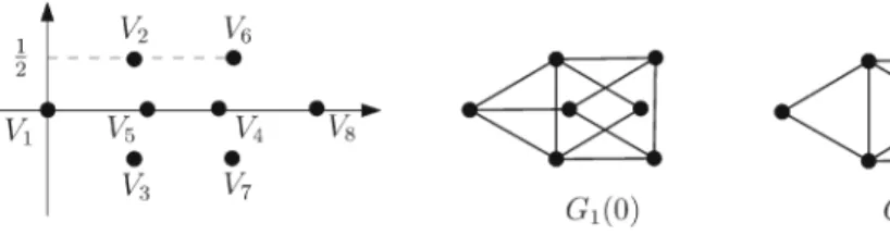
Fig. 1 The unit distance graphsG1(θ)andG2(θ)forθ=0
twoGx’s. Also, the density ofGxis f(x), andδ(A)= f(0), by definition. Therefore,
x∈G f(x)≤2f(0)+◦3(G).
We now turn to defining the geometric configurations to which inequalities (T1) and (T2) will be applied. Note that while the statements of Lemmas3.1 and3.2 are fairly trivial, it is not straightforward to find some geometric configurations such that conditions (T1) and (T2) yield non-trivial new constraints on the autocorrelation function f(x). The search for such configurations is almost like looking for a needle in a haystack, and we cannot point out any general method to succeed.
Letθ ∈ [0,2π]and consider the following eight points in the plane (see Fig.1):
V1 = (0,0), V2 = (√
3/2,1/2), V3 = (√
3/2,−1/2), V4 = (√
3,0), V5 = (cosθ,sinθ),V6=(√
3/2+cosθ,1/2+sinθ),V7=(√
3/2+cosθ,−1/2+sinθ), V8=(√
3+cosθ,sinθ). Consider the two unit distance graphs with vertex sets
G1=G1(θ)= {V1,V2,V3,V4,V5,V6,V7} and (5) G2=G2(θ)= {V1,V2,V3,V4,V6,V7,V8}, (6) and all pairs of vertices at distance 1 being connected with an edge. Notice that for all values ofθ, bothG1andG2have independence numberα=3, and both of them contain the same two independent triangles:(V1,V4,V6)and(V1,V4,V7). Therefore, 3(G1)=3(G2), which we commonly denote by3. We apply Lemma3.1toG1
to obtain
3 ≤ 1−7f(0)+
{x,y}∈(G21)
f(x−y),
while Lemma3.2applied toG2implies that
3≥
x∈G2
f(x)−2f(0).
Comparing these two estimates leads to
x∈G2
f(x) ≤ 1−5f(0) +
{x,y}∈(G21)
f(x−y). (CT)
This constraint turns out to be surprisingly powerful.
It is natural to wonder whether sharper bounds onm1(R2)could be reached by imposing further conditions on f, possibly coming from 4-tuple, 5-tuple, etc., corre- lations of the set A. The answer is provided by Theorems 1.1 and 7.3 in [5], which state that if we write up allcomplete positivity constraintsor allBoolean quadratic constraintson the function f, then the implied upper bound on the density of Awill converge tom1(R2). This means, in theory, thatthis method is guaranteed to succeed in proving the conjecturem1(R2) <0.25, if the inequality is true. In practice, however, the Boolean quadratic cone has so many facets even in relatively small dimensions that it is hopeless to add them all in any kind of numerical computation. For this rea- son, one is restricted to finding “clever” new constraints by geometric intuition, such as (CT) above. In comparison, we are not aware of such a theoretical guarantee of success for the method of fractional chromatic numbers of [3]: as far as we know, it may well happen that the fractional chromatic number of any finite unit distance graph is smaller than 4, whilem1(R2) <0.25.
4 Fourier Analysis and Linear Programming
A detailed description of the Fourier analytic method can be found in [8], we will only summarize the essentials here. We remind the reader that the 1-avoiding setAis assumed to be periodic with a period lattice L. This enables us to perform a Fourier expansion of f(x)=δ(A∩(A−x))in the Hilbert spaceL2(R2/L).
We also apply a standard trick of averaging. Note that all the inequalities stated in constraints (C1), (C2), (C1R), and (CT) hold for all rotated copies of a given graph.
Thus, they may be averaged over the orthogonal groupO(2)of the plane. We will use the notation ˚f(x)for the radial average of f(x):
f˚(x)= 1 2π S1
f(ξ|x|)dω(ξ), (7)
whereωis the perimeter measure on the unit circleS1. The advantage of this averaging is that ˚f is radial, i.e., ˚f(x)depends only on|x|. Also, the above remark shows that the constraints (C1), (C2), (C1R), and (CT) remain valid for the function ˚f.
As usual, the Bessel function of the first kind with parameter 0,2(|x|), is defined as
2(|x|)= 1 2π S1
ei xξdω(ξ).
As explained in [8],
f˚(x) =
u∈2πL∗
f(u)2(|u||x|),
whereL∗denotes the dual lattice ofL. Introducing the notation
κ(t) =
u∈2πL∗,|u|=t
f(u),
the previous equation simplifies to f˚(x)=
t≥0
κ(t)2(t|x|), (8)
where the summation is taken for those values oft which come up as a length of a vector in 2πL∗.
Introduce the notations δ = δ(A) andκ(t)˜ = κ(t)/δ. Conditions f(x) ≥ 0, f(0)=δ, (C0), (C1R), and (CT) via (7) and (8) lead to the following properties of the functionκ(t)˜ (see [8] for details):
(CP) κ(t)˜ ≥0 for everyt ≥0;
(CS)
t≥0κ(˜ t)=1;
(C0)
t≥0κ(t)˜ 2(t)=0;
(C1R) for every finite graphG,
t≥0
˜ κ(t)
⎛
⎝
x∈G
2(t|x|) −
{x,y}∈E(G)
2(t|x−y|)
⎞
⎠≤ α(G);
(CT) for any θ ∈ [0,2π], and the graphsG1(θ)andG2(θ)defined in Sect.3by (5) and (6),
t≥0
˜ κ(t)
⎛
⎜⎝
{x,y}∈(G21)
2(t|x−y|)−
x∈G2
2(t|x|)
⎞
⎟⎠≥ 5−1 δ.
Forget, for a moment, thatδ=δ(A)and just fix any particular value ofδ >0. Consider the coefficientsκ(t˜ )(fort ≥0) as variables in the continuous linear program
maximizeκ(0)˜ subject to(CP), ( CS), ( C0), ( C1R), (CT). (9) Lets =supκ(0)˜ denote the solution of this LP-problem. If, for a given value ofδ, there exists a 1-avoiding set Awith densityδ, then there exists a system of values
˜
κ(t)satisfying (9) such thatκ(0)˜ =δ. Therefore, in such a case,s ≥δ. Conversely, if for a given value ofδwe find thats< δ, then we may conclude that no 1-avoiding set with densityδexists, therefore,m1(R2)≤δ. By linear programming duality, the inequalitys< δmay be testified by the existence of a witness function.
Proposition 4.1 LetGbe a finite family of finite graphs inR2,T be a finite collection of angles in[0,2π], and for eachθ ∈T consider the unit distance graphs G1(θ),G2(θ)
defined in Sect.3by(5)and(6). Suppose that for some non-negative numbersv0,v1, wG for G∈G, andwθ forθ∈T, the function W(t)defined by
W(t)=v0+v12(t)+
G∈G
wG
⎛
⎝
x∈G
2(t|x|)−
{x,y}∈E(G)
2(t|x−y|)
⎞
⎠
−
θ∈T
wθ
⎛
⎜⎝
{x,y}∈(G1(θ)2 )
2(t|x−y|)−
x∈G2(θ)
2(t|x|)
⎞
⎟⎠
(10)
satisfies W(0)≥1and W(t)≥0for t>0. Then m1(R2)≤δ, whereδis the positive solution of the equation
δ2=δ
⎛
⎝v0+
G∈G
wGα(G)−5
θ∈T
wθ
⎞
⎠+
θ∈T
wθ. (11)
Proof For any functionW(t)satisfyingW(0)≥1 andW(t)≥0 fort >0 we have δ= ˜κ(0)≤
t≥0
˜
κ(t)W(t). (12)
IfW(t)is of the form (10), then inequalities(CP), (CS), (C0), (C1R), and (12) imply δ≤v0+
G∈G
wGα(G)−5
θ∈T
wθ+1 δ
θ∈T
wθ. (13)
5 Numerical Bounds
As indicated in Proposition4.1above, we will use two types of constraints, (C1R) and (CT), in addition to the trivial ones. Constraint (C1R) will be applied to certain isosceles triangles in the plane. Constraint (CT) will be applied, with particular choices of the angleθ, to the graphsG1(θ),G2(θ)defined by (5) and (6).
In order to handle the linear program numerically, we use a discrete approximation.
Based on the previous results, we only search for the coefficientsκ(t˜ i), whereti =iε0, withε0=0.05 andi ≤12000, thus,ti ∈ [0,600]. For all other values oft ≥0, we setκ(t˜ )=0. The error resulting from the discretization is corrected in the last step of the algorithm.
Finding suitable triangles and graphs which yield strong upper bounds onm1(R2)is a tedious task, where we utilized a bootstrap algorithm. Once a given set of constraints is fixed, and the corresponding linear program is solved, one has to numerically search for configurations of points for which (C1R) or (CT) is violated. Adding these to the list
0 1 2 3 4 5 0.05
0.10 0.15 0.20 0.25
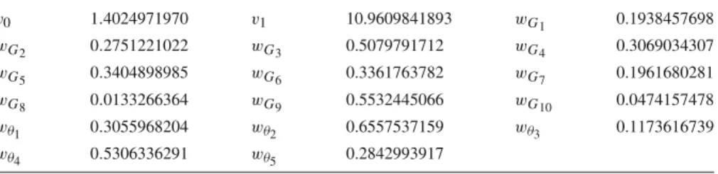
Fig. 2 The function ˚f(x)/δ
of constraints, and dropping the non-binding ones, the same procedure may be repeated until no significant improvement is obtained. In its polished form, our construction uses 15 nontrivial linear constraints: ten of the type (C1R) and five of type (CT).
The family G used for the estimate consists of ten triangles of the form {(x1,0), (x2,y), (x2,−y)}, with the triples(x1,x2,y)being listed in Table1. Con- straint (CT) is applied to the graphs defined by (5) and (6) with the values ofθranging over the familyT, which is listed in Table3. In order to avoid errors stemming from numerical computations, all the non-zero norms and distances between points of the configurations are chosen to be at least 0.1.
Using these graphs, we construct the witness function W(t)as in (10) with the coefficients described in Table4. It is easy to check numerically thatW(t)satisfies the required properties. Technical details about the rigorous verification of this are described in [8]. With this construction ofW(t), the quadratic equation (11) takes the form
δ2+7.188702δ−1.893645=0, whose positive solution isδ=0.254416.
The coefficientsκ(t˜ )obtained as the solution of the linear program (9) also pro- vide the normalized, radialized autocorrelation function ˚f(x)/δvia (8). This function could, in principle, be the autocorrelation of a hypothetical 1-avoiding set A with densityδ=0.254416. The function is plotted in Fig.2.
Acknowledgements The authors are grateful to Fernando M. de Oliveira Filho and Thomas Bellitto for the inspiring conversations, and to the anonymous referee for providing helpful suggestions.
Funding Open access funding provided by ELKH Alfréd Rényi Institute of Mathematics.
Open Access This article is licensed under a Creative Commons Attribution 4.0 International License, which permits use, sharing, adaptation, distribution and reproduction in any medium or format, as long as you give appropriate credit to the original author(s) and the source, provide a link to the Creative Commons licence, and indicate if changes were made. The images or other third party material in this article are included
in the article’s Creative Commons licence, unless indicated otherwise in a credit line to the material. If material is not included in the article’s Creative Commons licence and your intended use is not permitted by statutory regulation or exceeds the permitted use, you will need to obtain permission directly from the copyright holder. To view a copy of this licence, visithttp://creativecommons.org/licenses/by/4.0/.
Appendix: Numerical Values See Tables1,2,3and4.
Table 1 Triples{x1,x2,y}corresponding to the familyG
G1 {−0.123996,1.946331,0.501521} G2 {−0.157711,0.542869,0.499760} G3 {0.553873,−0.276937,0.479669} G4 {−0.424898,0.382590,0.490199} G5 {2.70637,1.842120,0.506318} G6 {−0.955984,0.026128,0.112481} G7 {−0.767499,0.143459,0.340280} G8 {0.476394,−0.337821,0.486967} G9 {0.668340,−0.199610,0.428893} G10 {−0.177622,0.519323,0.499597}
Table 2 Angles in the familyT
θ1 1.851176 θ2 1.864223 θ3 1.911210 θ4 1.935475 θ5 1.954980
Table 3 Angles in the familyT
θ1 1.851176 θ2 1.864223 θ3 1.911210 θ4 1.935475 θ5 1.954980
Table 4 Coefficients of the witness functionW(t)
v0 1.4024971970 v1 10.9609841893 wG1 0.1938457698
wG2 0.2751221022 wG3 0.5079791712 wG4 0.3069034307
wG5 0.3404898985 wG6 0.3361763782 wG7 0.1961680281
wG8 0.0133266364 wG9 0.5532445066 wG10 0.0474157478
wθ1 0.3055968204 wθ2 0.6557537159 wθ3 0.1173616739
wθ4 0.5306336291 wθ5 0.2842993917
References
1. Bachoc, Ch., Passuello, A., Thiery, A.: The density of sets avoiding distance 1 in Euclidean space.
Discrete Comput. Geom.53(4), 783–808 (2015)
2. Bellitto, T.: Walks, Transitions and Geometric Distances in Graphs. PhD thesis, Université de Bordeaux (2018).https://www.labri.fr/perso/tbellitt/tmp/thesis.pdf
3. Bellitto, T., Pêcher, A., Sédillot, A.: On the density of sets of the Euclidean plane avoiding distance 1 (2018).arXiv:1810.00960
4. Croft, H.T.: Incidence incidents. Eureka30, 22–26 (1967)
5. DeCorte, E., de Oliveira Filho, F.M., Vallentin, F.: Complete positivity and distance-avoiding sets.
Math. Program. (2020).https://doi.org/10.1007/s10107-020-01562-6
6. Erd˝os, P.: Problems and results in combinatorial geometry. In: Discrete Geometry and Convexity (New York 1982). Annals of the New York Academy of Sciences, vol. 440, pp. 1–11. New York Academy of Sciences, New York (1985)
7. de Grey, A.D.N.J.: The chromatic number of the plane is at least 5. Geombinatorics28(1), 18–31 (2018)
8. Keleti, T., Matolcsi, M., de Oliveira Filho, F.M., Ruzsa, I.Z.: Better bounds for planar sets avoiding unit distances. Discrete Comput. Geom.55(3), 642–661 (2016)
9. Moser, L., Moser, W.: Solution to problem 10. Can. Math. Bull.4(2), 187–189 (1961)
10. de Oliveira Filho, F.M., Vallentin, F.: Fourier analysis, linear programming, and densities of distance avoiding sets inRn. J. Eur. Math. Soc.12(6), 1417–1428 (2010)
11. Székely, L.A.: Erd˝os on unit distances and the Szemerédi–Trotter theorems. In: Paul Erd˝os and His Mathematics (Budapest 1999), vol. 2. Bolyai Soc. Math. Stud., vol. 11, pp. 649–666. Springer, Berlin (2002)
Publisher’s Note Springer Nature remains neutral with regard to jurisdictional claims in published maps and institutional affiliations.