Minimal sets and chaos in
planar piecewise smooth vector fields
Tiago Carvalho
B1and Rodrigo Donizete Euzébio
21Departamento de Computação e Matemática, Faculdade de Filosofia, Ciências e Letras de Ribeirão Preto, USP, Av. Bandeirantes, Zip Code 14098-322, Ribeirão Preto, SP, Brazil
2Departamento de Matemática, IME–UFG, R. Jacarandá, Campus Samambaia, Zip Code 74001-970, Goiânia, GO, Brazil
Received 17 May 2019, appeared 20 May 2020 Communicated by Armengol Gasull
Abstract. Some aspects concerning chaos and minimal sets in discontinuous dynamical systems are addressed. The orientability dependence of trajectories sliding trough some variety is exploited and new phenomena emerging from this situation are highlighted.
In particular, although chaotic flows and nontrivial minimal sets are not allowed for smooth vector fields in the plane, the existence of such objects for some classes of vector fields is verified. A characterization of chaotic flows in terms of orientable minimal sets is also provided. The main feature of the dynamical systems under study is related to the non uniqueness of trajectories in some zero measure region as well as the orientation of orbits reaching such region.
Keywords: vector fields, piecewise smooth vector fields, chaos, minimal sets.
2020 Mathematics Subject Classification: 34C28, 37D45.
1 Introduction
Dynamical systems have become one of the most promising areas of mathematics since its strong development started by Poincaré (see [22]). The main reason for this is due to the fact that several applied sciences from economy and biology to engineering and statistical mechan- ics benefited of dynamical systems’ tools. In the last case, for instance, ergodic theory plays an important role, we mention for short Poincaré recurrence theorem as well as the concepts of chaos and entropy. In fact, while a mathematical object models a concrete phenomena, such modeling is in fact no more than an theoretical approximation of an real event and invariably ignores some important features of it. Is therefore mandatory to search for news methods and tools that are not only more realistic but also feasible in theory.
In this direction have emerged within the theory of dynamical system a set of methods which is now widely known by piecewise smooth vector fields (PSVFs, for short). For a formal introduction to PSVFs see [14]. The main advantage of PSVFs over the classical theory of
BCorresponding author. Email: tiagocarvalho@usp.br
dynamical system is the fact that they provide a more accurate approach by allowing non smoothness or discontinuities of the vector field defining the system. Indeed, several prob- lems involving impact, friction or abrupt changes of certain regime can be modeled or at least approximated by PSVFs, in the sense that the transition from one kind of behavior to another one can be idealized as a discrete and instantaneous transition. A non exhaustive list of ap- plications of such theory involves the relay systems, the control theory, the stick-slip process, the dynamics of a bouncing ball and the antilock braking system (ABS), see those and other applications in [2–4,11,12,15,16,18,19] and references therein.
The main aspect of PSVFs concerns non uniqueness of solutions on some zero measure variety and consequent amalgamation of orbits under such region, which split the phase por- trait into two or more pieces. That leads to the behavior known assliding motion, characterized by the collapse of distinct trajectories which combine to slide on the common frontier of each dynamic. Under this scenario some behavior strange to the classical theory of dynamical sys- tems may occur, so the study of new objects and the validation of known results is mandatory when one investigate PSVFs. For instance, we mention the Peixoto‘s Theorem (see [21]), the Closing Lemma (see [8]) and the Poincaré–Bendixson Theorem (see [5]), which posses ana- logues version in the context of PSVFs (see also [10,13,17]). We also mention that the study of PSVFs may take into account orientability of trajectories. This is because the collision of any particular trajectory to the boundary region and subsequent sliding occurs in different ways when considering forward or backward time.
This paper is addressed to some particular features of PSVFs. Indeed, we take into ac- count aspects of chaotic PSVFs and how this concept relates to minimal sets. To do this, the definitions of both chaos e minimal sets are refined to consider the role of orientation and we provide a definitive characterization of chaotic PSVFs involving such objects.
Let med(W)be the Lebesgue measure of a setW. The first main result of the paper states thata PSVF Z is chaotic on the set W if, and only if, Z is positive chaotic and negative chaotic on W.
The second main result of the paper states that if Z is chaotic on the set W andmed(W) > 0 then W is positive minimal and negative minimal. In order to prove these results we present and prove some other results which are indispensable to main results but also important on their own. For instance, we provide a sufficient condition for a Lebesgue measure subset of R2 to be chaotic, which elucidates the richness of PSVFs. Other considerations and results are presented timely throughout the text.
The paper is organized as follows: in Section2we provide the first statements around the subject of PSVFs, particularly considering minimal sets for PSVFs and their chaotic behavior.
In Section 3 we state and prove the main results of the paper and some consequences of them. In Section4we provide a discussion around the results of the paper and present some examples and counterexamples contextualizing the results.
2 Preliminaries
2.1 Piecewise smooth vector fields
Consider two smooth vector fields X and Y and a codimension one manifold Σ ⊂ R2 that separates the plane in two regionsΣ+ andΣ−. A PSVFZis a vector field defined inR2and
given by
Z(x,y) =
(X(x,y), for(x,y)∈Σ+,
Y(x,y), for(x,y)∈Σ−. (2.1) SinceΣis a codimension one manifold, there exists a function fsuch thatΣ= f−1(0)and 0 is a regular value of f. As consequence,Σ+= {q∈R2|f(q)≥0}andΣ−= {q∈R2|f(q)≤ 0}. The trajectories of Z are solutions of ˙q = Z(q) and we accept it to be multi-valued at points ofΣ. We will callΩthe set of all PSVFs defined inR2. The basic results of differential equations in this context were stated by Filippov in [14], that we summarize next. Indeed, consider the Lie derivatives X.f(p) = h∇f(p),X(p)i and Xi.f(p) = ∇Xi−1.f(p),X(p), i ≥ 2, where h., .iis the usual inner product in R2. We distinguish the following regions on the discontinuity set Σ:
(i) Σc ⊆ Σ is the sewing regionif (X.f)(Y.f) > 0 on Σc. Moreover, when X.f(p) > 0 and Y.f(p) > 0, we say that p ∈ Σc+ and when X.f(p) < 0 and Y.f(p) < 0, we say that p∈ Σc−.
(ii) Σe⊆Σis theescaping regionif (X.f)>0 and(Y.f)<0 on Σe. (iii) Σs⊆Σis thesliding regionif(X.f)<0 and(Y.f)>0 on Σs.
Thesliding vector fieldassociated toZ ∈ Ωis the vector fieldZs tangent toΣs and defined at q ∈ Σs by Zs(q) = m−q with m being the point of the segment joining q+X(q) and q+Y(q)such thatm−qis tangent toΣs. It is clear that ifq∈Σsthenq∈Σefor(−Z)and we can define the escaping vector field Ze on Σe associated toZ byZe = −(−Z)s. We will use the notationZΣ to both,ZsandZe.
We say thatq∈Σis aΣ-regular pointif it is a sewing point or a regular point of the Filippov vector field. Lastly, any point q∈Σp is called apseudo-equilibrium of Z and it is characterized by ZΣ(q) = 0. Any q ∈ Σt is called a tangential singularity (or also tangency point) and it is characterized by (X.f(q))(Y.f(q)) =0. If there exist an orbit of the vector field X|Σ+ (respec.
Y|Σ−) reaching q ∈ Σt in a finite time, then such tangency is called a visible tangency for X (resp.Y); otherwise we callqaninvisible tangencyforX (resp.Y).
We may also distinguish a particular tangential singularity calledtwo-fold, which is a com- mon tangencyqof bothXandY(that is,X.f(q) =Y.f(q) =0) satisfyingX2.f(q)),Y2.f(q))6=
0. A two-fold is called visible if it is a visible tangency for X and Y. A visible two fold singularity is called a singular tangency pointand all other p ∈ Σt is called a regular tangency point.
Definition 2.1. Thelocal trajectory (orbit)φZ(t,p)of a PSVF given by (2.1) throughp∈R2is defined as follows:
(i) For p∈Σ+\Σandp∈Σ−\Σthe trajectory is given byφZ(t,p) =φX(t,p)andφZ(t,p) = φY(t,p)respectively, wheret∈ I : the maximal interval of existence of the corresponding trajectory before it hits Σ.
(ii) For p ∈ Σc+ and taking the origin of time at p, the trajectory is defined as φZ(t,p) = φY(t,p) for t ∈ I∩ {t ≤ 0} and φZ(t,p) = φX(t,p) for t ∈ I ∩ {t ≥ 0}. For the case p ∈ Σc− the definition is the same reversing time. Again, I is the maximal interval of existence of the corresponding trajectory before it hitsΣagain.
(iii) For p ∈ Σe and taking the origin of time at p, the trajectory is defined as φZ(t,p) = φZΣ(t,p) for t ∈ I ∩ {t ≤ 0} and φZ(t,p) is either φX(t,p) or φY(t,p) or φZΣ(t,p) for t ∈ I∩ {t ≥ 0}. For p ∈ Σs the definition is the same reversing time. Here, I is the maximal interval of existence of the corresponding trajectory ofφX(t,p)or φY(t,p) before it hitsΣagain orφZΣ(t,p)before it leavesΣ.
(iv) Forpa regular tangency point and taking the origin of time at p, the trajectory is defined asφZ(t,p) =φ1(t,p)fort ∈ I∩ {t≤0}andφZ(t,p) =φ2(t,p)fort∈ I∩ {t≥0}, where eachφ1,φ2 is either φX or φY or φZT. Here, I is the maximal interval of existence of the corresponding trajectory ofφX(t,p)or φY(t,p)before it hitsΣagain or φZΣ(t,p)before it leavesΣ.
(v) For pa singular tangency point,φZ(t,p) =pfor all t∈R.
Definition 2.2. Letφ1Z andφ2Z two distinct local trajectories. Suppose that there exists a com- mon pointq∈ φ1Z∩φ2Z. We say thatφ1Z∪φ2Z preserves orientation if there exists an interval I, with 0 ∈ I, such that: (i) φZ1(0,q) =φ2Z(0,q), (ii) φZ1(t, .) is well defined fort ∈ I∩ {t ≤ 0} and (iii)φ2Z(t, .)is well defined fort∈ I∩ {t≥0}.
Remark 2.3. Note that the pointqof the previous definition is such that q ∈ Σ. In fact, it is enough to observe that there is uniqueness of trajectories in points belonging toR2\Σ.
Definition 2.4. Aglobal trajectory (orbit)ΓZ(t,p0)of Z∈Ωpassing through p0 whent =0, is a unionΓZ(t,p0) =∪i∈Θ{σi(t,pi);ti ≤ t ≤ ti+1}of preserving-orientation local trajectories σi(t,pi) satisfying σi(ti,pi) = pi ∈ Σ and σi(ti+1,pi) = pi+1 ∈ Σ, here Θ ⊂ Z. A maximal trajectory ΓZ(t,p0)is a maximal trajectory that cannot be extended to any others global tra- jectories by joining local ones, that is, ifeΓZ is a global trajectory containingΓZ then eΓZ = ΓZ. In this case, we callI = (τ−(p0),τ+(p0))themaximal interval of the solutionΓZ. A maximal trajectory is apositive(respectively, negative) maximal trajectory if we restrict the previous definition tot ≥0 (resp. t ≤0).
Definition 2.5. A maximal trajectory ΓZ(t,p0) has a positive (respectively, negative) peri- odic trajectory passing through p0 if there exists T+ > 0 (respectively, T− > 0) such that φZ(t+k T+,p0) =φZ(t,p0)for all integer k > 0 (respectively,φZ(t+k T−,p0) =φZ(t,p0)for all integer k < 0). A maximal trajectory ΓZ(t,p0) has aperiodic trajectory passing through p0 if it has coincident positive and negative periodic trajectories passing throughp0in such a way thatT+= T−.
Definition 2.6. Consider Z = (X,Y) ∈ Ω. A closed (connected) union of trajectories ∆ of Z is a:
(i) pseudo-cycle if ∆∩Σ 6= ∅ and it does not contain neither equilibrium nor pseudo- equilibrium.
(ii) pseudo-graphif ∆∩Σ6= ∅and it is a union of equilibria, pseudo equilibria and orbit- arcs ofZjoining these points.
2.2 Minimal sets and chaotic PSVFs
One of the most important facts concerning PSVFs is the orientation of its trajectories. Indeed, it is very important, for instance, for the concept of invariance or defining the flow associated
to the Filippov vector field. In the smooth theory of vector fields this distinction does not play an important role since we have uniqueness of trajectories. In this direction, we should verify if such distinction is also necessary when defining minimal sets and chaotic PSVFs. Indeed, these concepts do not play the same role by considering positive and negative times. As far as the authors know, the role of orientability under this context have not be treated in literature about PSVFs, although the concept of chaos and minimality have been discussed before, for instance, in [5], [6] and [10]. We start doing some adaptations to the definitions of invariance and minimality.
Definition 2.7. A setA⊂R2ispositive invariant(respectively,negative invariant) if for each p ∈ A and all positive maximal trajectoryΓ+Z(t,p)(respectively, negative maximal trajectory Γ−Z(t,p)) passing through pit holdsΓ+Z(t,p)⊂ A(respectively,Γ−Z(t,p)⊂ A). A set A⊂R2is invariantforZif it is positive and negative invariant.
Definition 2.8. Consider Z ∈ Ω. A non-empty set M ⊂ R2 is minimal(respectively, either positive minimal or negative minimal) for Z if it is compact, invariant (respectively, either positive invariant or negative invariant) for Zand does not contain proper compact invariant (respectively, either does not contain proper compact positive invariant or proper compact negative invariant) subsets.
Next we present the definitions concerning chaotic PSVFs. As commented before, we need to distinguish between forward and backward time or assuming both possibilities. The notion of chaos we take into account is that based on Devaney. So, the first aspect to be considered is related to topological transitivity.
Definition 2.9. System (2.1) istopologically transitiveon an invariant setW if for every pair of nonempty, open sets U and V in W, there exist q+,q− ∈ U, Γ+Z(.,q+),Γ−Z(.,q−) maximal trajectories andt+0 >0>t−0 such thatΓ+Z(t+0,q+)andΓ−Z(t−0,q−)∈V.
Definition 2.10. System (2.1) is topologically positive transitive(respectively, topologically negative transitive) on a positive invariant (respectively, negative invariant) setW if for every pair of nonempty, open setsUandVinW, there existq∈ U,Γ+Z(t,q)a positive (respectively, Γ−Z(t,q)a negative) maximal trajectory andt0>0 (resp.,t0 <0) such thatΓ+Z(t0,q)∈V(resp., Γ−Z(t0,q)∈V).
Remark 2.11. A direct consequence of the two previous definitions is that:
Zis topologically transitive onW if, and only if, Zis simultaneously topologically positive transitive and topologically negative transitive onW.
Analogously to the definition of topologically transitive systems, the definition of sensitive dependence for PSVFs is inspired in the classical Devaney concept of chaos.
Definition 2.12. System (2.1) exhibits sensitive dependenceon a compact invariant setW if there is a fixedr >0 satisfyingr < diam(W)such that for each x ∈ W andε > 0 there exist y+,y− ∈ Bε(x)∩W and maximal trajectoriesΓ+x, Γ−x, Γ+y+ and Γ−y− passing through x, y+ and y−, respectively, satisfying
dH(Γ+x(t),Γ+y+(t)) = sup
a∈Γ+x(t),b∈Γ+y+(t)
d(a,b)>r,
dH(Γ−x(t),Γ−y−(t)) = sup
a∈Γ−x(t),b∈Γ−
y−(t)
d(a,b)>r,
where diam(W)is the diameter ofW anddis the Euclidean distance.
Associated to the previous definition we give the next one, where the orientation of the trajectories ofZis also considered:
Definition 2.13. System (2.1) exhibitssensitive positive dependence(resp.,sensitive negative dependence) on a compact positive invariant (resp., negative invariant) setWif there is a fixed r> 0 satisfyingr <diam(W)such that for eachx ∈W andε >0 there exist a y∈ Bε(x)∩W and positive (resp., negative) maximal trajectories Γ+x and Γ+y (resp., Γ−x and Γ−y) passing throughx andy, respectively, satisfying
dH(Γ+x(t),Γ+y(t)) = sup
a∈Γ+x(t),b∈Γ+y(t)
d(a,b)>r,
(resp.,dH(Γ−x(t),Γ−y(t)) = sup
a∈Γ−x(t),b∈Γ−y(t)
d(a,b)>r),
where diam(W)is the diameter ofW andd is the Euclidean distance.
Remark 2.14. A direct consequence of the two previous definitions is that:
Zexhibits sensitive dependence onW if, and only if,Zexhibits simultaneously sensitive positive dependence and sensitive negative dependence onW.
In this paper we will consider the notations stated in the following table.
Table of abbreviations
Topologically transitive TT Topologically positive transitive TPT Topologically negative transitive TNT Sensitive dependence SD Sensitive positive dependence SPD Sensitive negative dependence SND
We should mention, as observed in [10], that Definitions 2.9 and 2.12 coincide with the definitions of topological transitivity and sensible dependence of smooth vector fields for single-valued flows, so these definitions are natural extension for a set-valued flow. Lastly, in what follows we introduce the definition of chaos and orientable chaos in the piecewise smooth context. Note that the concept for chaos in the paper is inspired by Devaney for a deterministic flow, but the systems of differential equations discussed in the article define non-deterministic flows:
Definition 2.15. System (2.1) ischaotic(resp., eitherpositive chaotic ornegative chaotic) on a compact invariant (resp., either positive invariant or negative invariant) setW if it is TT and exhibits SD (resp., either TPT and exhibits SPD or TNT and exhibits SND) onW.
Remark 2.16. A direct consequence of the previous definition is that:
A PSVFZis chaotic onW if, and only if,Zis positive chaotic and negative chaotic onW.
3 Main results
In this Section we present and prove the main results of the paper.
Proposition 3.1. LetAbe the set of pseudo cyclesΓof Z= (X,Y)such thatΓ∩(Σe∪Σs) =∅and Γhas at least a visible two-fold singularity. The elementsΓofAare chaotic for Z.
In Figure4.5 we exhibit an element Γ ⊂ A. In fact, the elements Γ ⊂ A are obtained by the concatenation of orbits ofXandY, without using orbits ofZΣ.
Proof of Proposition3.1. Let A,Bopen sets relative toΓ. SinceΓis a pseudo-cycle, given points pA ∈ A and pB ∈ B, there exists a trajectory of Zconnecting them (for positive and negative times). SoΓis topologically transitive.
On the other hand, givenx,y∈ A, there exists a trajectory passing throughxand another trajectory passing throughysuch that each one of them follows a distinct path after the visible two-fold singularity ofΓ. SoΓhas sensitive dependence.
Therefore,Γis chaotic.
Remark 3.2. By the previous proposition, we conclude the existence of trivial minimal sets presenting chaotic behavior.
Remark 3.3. An analogous of result of Remarks2.11,2.14and2.16does not hold for minimal sets. Indeed, while sets which are both positive and negative minimal are also minimal, the converse is not true. The Example 2 of [6] exemplify this situation.
The most part of the results obtained in [5] and [6] takes into account sets having positive Lebesgue measure. Indeed, in almost every approach concerning ergodic aspects of PSVFs, this is the interesting case. We cite, for instance, the existence of non-trivial minimal sets and planar chaotic PSVFs, as shown in the papers cited previously. In this direction we state the next result.
Lemma 3.4. Let K ⊂ R2 be a compact invariant set and Z a PSVF presenting a finite number of critical points and a finite number of tangency points withΣin K. Ifmed(K) =0and K6∈ Athen Z is not chaotic on K.
We recall that A is the set of pseudo-cycles having a visible two-fold singularity which does not connect to any sliding or escaping segment (see Proposition3.1). Also, thesaturation of a set M by a vector fieldW is the set
W(M) ={φW(t,p)| p∈ Mandt∈ I}
where I is the maximal interval of existence of theW-trajectory passing throughp.
Proof. First, suppose that K∩Σ ⊂ Σc∪Σt and take p ∈ K. Consequently, φZ(t,p) −−→t→∞ L ∈ ω(p) ⊂ K, since K is compact. Here ω(p) denotes the ω-limit set of the point p.
Thus, by using the Poincaré–Bendixson Theorem for PSVFs (see [5]) we get that L is a (pseudo-)equilibrium, a (pseudo-)graph or (pseudo-)cycle which does not belongs toAsince L⊂KandK6∈ Aby hypothesis. In any case, it is trivial to see thatZis not chaotic onKsince Zdoes not exhibits SD onK.
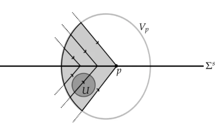
Now consider the case where K∩(Σs∪Σe) 6= ∅ and suppose that there exist a PSVF Z which is chaotic onK. Takep∈K∩(Σs∪Σe)andVp ⊂R2a neighborhood ofp. Consider the
sets Vp+ = {φ+t (p)∩Vp|φ+t is a positive trajectory ofZpassing through p} and Vp− defined analogously for the negative trajectory. Observe that med(Vp+∪Vp−) > 0, since using the Definition2.1, in this case the saturation ofK∩(Σs∪Σe)(for either positive or negative times) contain an open set U ⊂ Vp satisfying 0 < med(U) < med(Vp+∪Vp−). Consequently there exist a point q ∈ Vp+∪Vp− such that q 6∈ K, because otherwise Vp+∪Vp− ⊂ K and then med(K)>med(Vp+∪Vp−)>0 (see Figure3.1). As consequence, Kis not invariant, producing a contradiction.
Vp
p Σs
U
Figure 3.1: The neighborhoodVpof p. The filled region correspond toVp−, and in this caseVp+ =Vp∩Σ. Observe that it has positive Lebesgue measure.
In the proof of the next Theorem3.6we will use the following remark.
Remark 3.5. A direct consequence of Definition2.15is that
LetZa chaotic PSVF onW. ThenZis chaotic on every compact invariant proper subset We ⊂W.
In [6], among other results, the authors prove that, if a compact invariant setW satisfying med(W)>0 is simultaneously positive and negative minimal for a PSVFZ, thenZis chaotic onW. Now, we prove the converse of this important theorem. Observe that, due to Lemma3.4, we must impose a condition demanding the positive Lebesgue measure of the considered set.
Theorem 3.6. If Z is chaotic on the compact invariant set W,med(W) > 0, Z has a finite number of critical points and a finite number of tangency points withΣin W, then W is positive minimal and negative minimal for Z.
Proof. According to Remark2.16,Zis positive chaotic onW. So,W is compact, non-empty and positive invariant. Suppose thatW is not positive minimal. In this case, there exists a proper subsetWe ofW with the previous three properties. Moreover, by Remark3.5 and Lemma3.4, we get med(We)> 0 or med(We) =0 andWe ⊂ A. Of courseWe is not dense inW since We is compact andWe 6= W. Therefore there exists an open set A ⊂W such that A∩We = ∅. First suppose that med(We)>0 and letB⊂We be an open set ofW. In this case, using the open sets
A andB, we have that Z is not TPT. But this is a contradiction with the fact thatZis chaotic on W. On the other hand, if med(We) = 0 we get We ⊂ A and thereforeWe is a curve on W. Let I(We)the region delimited byWe which is clearly invariant and notice that med(I(We))>0 since med(We) = 0. So we can take open sets B ⊂ I(We) and A ⊂ W\ We ∪I(We) to lead again to a contradiction with the fact that Zis chaotic onW. Therefore,W is positive minimal forZ.
An analogous argument proves thatW is negative minimal forZ.
Next corollary is a straightforward consequence of Theorem 3.6, but it is very important once it provides a ultimate answer about the relation between chaotic systems and minimal sets.
Corollary 3.7. If Z is chaotic on W,med(W)>0, Z has a finite number of critical points and a finite number of tangency points with Σin W, then W is minimal for Z.
Proof. It is enough to use Theorem3.6and Definition2.8.
We remark that the converse is not true, as observed in [6].
The next two corollaries are also consequences of Theorem3.6. Their proofs, analogously, are quite trivial although the results can find applications.
Corollary 3.8. If med(W) > 0, Z has a pseudo equilibria on W and a finite number of tangency points with Σin W then Z is not chaotic on W.
Proof. It is not difficult to see that a pseudo equilibria is neither positive nor negative minimal for Z since there exists trajectories of X andY hitting it in finite (positive or negative) time.
So, W is not positive or negative minimal. Therefore the proof follows straightforward from Theorem3.6.
Remark 3.9. A consequence of the proof of Theorem3.6is that
IfZis positive (resp. negative) chaotic onW, med(W)>0, Zhas a finite number of tangency points withΣinW thenW is positive (resp. negative) minimal.
The next result provide a sufficient condition in order to a PSVF Z be chaotic on an in- variant compact setW. Additionally, it guarantee that under suitable hypotheses the periodic trajectories of Zare dense inW.
Theorem 3.10. Let Z be a PSVF and W a compact positive (resp. negative) invariant set satisfying med(W) > 0. Given x,y ∈ W, assume that there exist a positive (resp. negative) trajectory φ+t (resp.φt−) connecting x and y. Then Z is positive (resp. negative) chaotic on W and the positive (resp.
negative) periodic trajectories of Z are dense in W.
We shall prove the last result in forward time, obtaining positive chaos and dense trajecto- ries. The proof for trajectories in backward time is completely similar.
Proof. Since med(W) > 0, let U and V be nonempty open sets in W and pU, pV points of U and V, respectively. By hypotheses there exist a positive trajectory φt+ connecting pU and pV in forward time. Since U and V are arbitrary it follows that W is topologically positive transitive. On the other hand, letdW be the diameter ofW and taker=dW/2, so clearly there existsa,b∈W such thatd(a,b)>r. Now considerx ∈W,ε>0 and fixy∈Bε(x)∩W. Again, by hypotheses there exists positive trajectories φ+a (t,x) and φb+(t,x) satisfying φ+a (0,x) =
φb+(0,x) = x and values ta,tb > 0 such that φ+a (ta,x) = a and φb+(tb,x) = b so Z exhibits sensitive positive dependence on W. At last, the density of positive periodic trajectories is straightforward from the fact that any point x ∈ W can be connected to itself by a positive trajectory.
Theorem3.10leads to the next corollary.
Corollary 3.11. Let Z be a PSVF and W satisfying med(W) > 0a compact invariant set on which any two points can be connected simultaneously by positive and negative trajectories. Then Z is chaotic on W and its periodic trajectories are dense in W.
Proof. Since every pair of points inW can be connected simultaneously by positive and nega- tive trajectories ofZ, by Theorem3.10, the PSVFZis both positive and negative chaotic on Z.
So, by Remark2.16, we get thatZ is chaotic onW. Moreover, since the positive and negative periodic trajectories ofZare dense inW, the density of the periodic trajectories of Zon W is straightforward.
4 Discussions
We observed throughout the paper a closed relation between PSVFs presenting minimal sets or chaotic behavior. However, in order to observe the richness of such relation we introduced new concepts by considering the orientation of the trajectories in time. By one hand, according to Theorem 14 of [6], every PSVF having a positive and negative non trivial minimal set Kis chaotic on K. On the other hand, in this paper, due to Remark 2.16 and 3.6 we get the equivalence. Putting those and other results of this paper together, we get the following diagram:
Z is pos. and
neg. chaotic onW ⇔ Zis chaotic
onW ⇔ W is pos. and
neg. min. forZ ⇒ W is min.
for Z
We note by observing the previous diagram that it could exist some minimal set which is not chaotic for the PSVF, as the authors observed in [5]. Other aspects of that diagram are presented in what follows:
Orientable chaotic sets which are not chaotic: Consider the PSVF:
ccZe(x,y) = (x, ˙˙ y) = 1 2
(−1,−2x−x2(4x+3) + (1+e)x(3x+2)) +sgn(y) (3,−2x+x2(4x+3)−(1+e)x(3x+2))
(4.1)
or, equivalently,
Ze(x,y) =
(X(x,y) = (1,−2x) ify≥0,
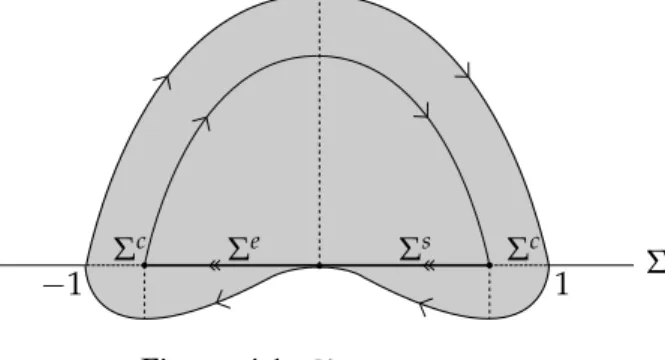
Ye(x,y) = (−2,−x2(4x+3) + (1+e)x(3x+2)) ify≤0, (4.2) withe∈ Ran arbitrarily small parameter. In [6] the authors proved thatZ0 has a chaotic set given (see Figure4.1) by
Λ={(x,y)∈R2| −1≤x ≤1 and x4/2−x2/2≤y≤1−x2}. (4.3)
Σe Σs
Σc Σc Σ
−1 1
Figure 4.1: Chaotic setΛ.
Taking e < 0 (resp., e > 0) in (4.2) the PSVF Ze has a negative chaotic (resp., positive chaotic) setΛ. We construct such a set for the casee ε <0. Indeed call p2 the two-fold located at the origin and p1 the first intersection of the backward trajectory of p2 with Σ. From p1 it can be concatenated a regular arc of trajectory of X which again intersects Σ in backward time at a point p4. Finally, call p3 the continuation of p4 through the trajectory of Y until reachingΣ. Hence the set Λe is the region bounded by [p1p2∪p[2p3∪[p3p4∪[p4p1, wherea bc is the orbit-arc connecting the points a and b, see the shadowed region in Figure4.2 (resp., Figure 4.3). Moreover, when e6= 0, Λe is not a chaotic set. This happens becauseΛe is not an invariant set; it is only negative invariant (resp., positive invariant).
p1 p2
p3 p4
Figure 4.2: Negative chaotic setΛ.e
p1 p2
p3 p4
Figure 4.3: Positive chaotic setΛ.e
Remark 4.1. The previous paragraph remains true if we change the word chaotic by the word minimal. A complete bifurcation analysis of the family (4.2) is given in [8].
The sets given in Figures 4.2 and 4.3 are orientable chaotic and orientable minimal sets.
Despite of this, it is easy to exhibit examples of orientable minimal sets that are not orientable chaotic.
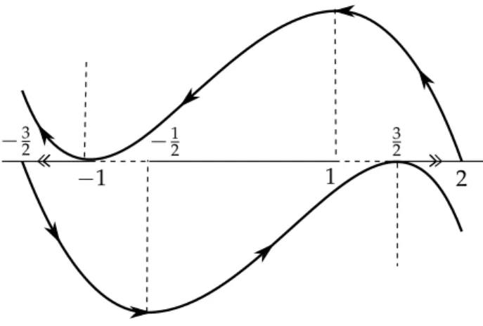
Orientable chaotic sets and orientable minimality: Consider the PSVF
Z(x,y) = (X(x,y),Y(x,y)) = ((−1, 3x2−3),(1,−(9/4) +3(−1+x)x)).
Such PSVF has a periodic orbit (see Figure4.4) which is a negative minimal set. However,Z is not a negative chaotic PSVF on the periodic orbit since it does not present SPD.
Observe that, in the last example the Lebesgue measure of the periodic orbit is null. How- ever, it is not difficult to exhibit a minimal set W for some PSVF, with med(W)> 0, in such way that W is neither positive chaotic nor negative chaotic. Indeed, Example 2 of [6] satis- fies these properties. In other words, in general minimality does not imply chaoticity. The converse, on the other hand, is true, as proved in Section3.
−32 −12
−1 1
3 2
2
Figure 4.4: Periodic orbit (for positive time).
Trivial chaos: In PSVFs the route to chaos is not hard. In fact, here we show that a chaotic behavior can be achieved by trivial minimal sets.
Consider the PSVF Z = (X,Y) where X(x,y) = (1, 4x(1 − x2)) and Y(x,y) = (−1, 4x(1−x2)). The phase portrait is pictured in Figure 4.5. Take Λ = Λ1∪Λ2, where Λ1(respectively, Λ2) is the trajectory of X(respectively,Y) passing through p1 = (−√
2, 0). It is easy to see thatΛis a trivial minimal set (a pseudo-cycle) and it is a chaotic set forZ.
p1 −1 0 1
Γ1
Γ2
Figure 4.5: Trivial minimal set which is chaotic forZ.
The previous example illustrates a more general result, stated in Proposition3.1.
We finish this section highlighting two particular conclusions from the results of the paper:
(i) although the chaoticity of a PSVFZunder a setW implies thatW is minimal for Z, the converse is false according to Example 2 of [6];
(ii) ifZis positive chaotic on W thenW is positive minimal for Z(see Remark3.9), but the converse is false since we can exhibit positive minimal sets that are not positive chaotic (see Example 4 in [5]). Analogously for negative chaotic/minimal.
Acknowledgment
The authors would like to thank the anonymous referees for their valuable comments which helped to improve the manuscript.
The first author is partially supported by grants #2017/00883-0 and #2019/10450-0, São Paulo Research Foundation (FAPESP) and by CNPq-BRAZIL grant 304809/2017-9. The sec- ond author is partially supported by Pronex/FAPEG/CNPq Proc. 2012 10 26 7000 803 and Proc. 2017 10 26 7000 508, Capes grant 88881.068462/2014-01 and Universal/CNPq grant 420858/2016-4.
References
[1] M. di Bernardo, C. J. Budd, A. R. Champneys, P. Kowalczyk, Piecewise-smooth dynam- ical systems. Theory and applications, Applied Mathematical Sciences, Vol. 163, Springer- Verlag London, Ltd., London, 2008. https://doi.org/10.4249/scholarpedia.4041;
MR2368310
[2] M. di Bernardo, A. Colombo, E. Fossas, Two-fold singularity in nonsmooth electrical systems, in: Proc. IEEE International Symposium on Circuits ans Systems, 2011, pp. 2713–
2716.https://doi.org/10.1109/ISCAS.2011.5938165
[3] M. di Bernardo, K. H. Johansson, F. Vasca, Self-oscillations and sliding in relay feedback systems: symmetry and bifurcations, Internat. J. Bifur. Chaos Appl. Sci. Engrg.
11(2001), 1121–1140.https://doi.org/10.1142/S0218127401002584
[4] B. Brogliato,Nonsmooth mechanics. Models, dynamics and control, Third edition, Commu- nications and Control Engineering Series. Springer-Verlag, 2016. https://doi.org/10.
1007/978-3-319-28664-8;MR3467591
[5] C. A. Buzzi, T. Carvalho, R. D. Euzébio, On Poincaré–Bendixson theorem and non- trivial minimal sets in planar nonsmooth vector fields, Publ. Mat. 62(2018), 113–131.
https://doi.org/10.5565/PUBLMAT6211806;MR3738185
[6] C. A. Buzzi, T. Carvalho, R. D. Euzébio, Chaotic planar piecewise smooth vector fields with non-trivial minimal sets, Ergodic Theory Dynam. Systems 36(2016), 458–469. https:
//doi.org/10.1017/etds.2014.67;MR3503032
[7] C. A. Buzzi, T. Carvalho, M. A. Teixeira, Birth of limit cycles bifurcating from a non- smooth center, J. Math. Pures Appl. (9) 102(2014), 36–47. https://doi.org/10.1016/j.
matpur.2013.10.013;MR3212247
[8] T. Carvalho, On the closing lemma for planar piecewise smooth vector fields, J. Math.
Pures Appl. (9)106(2016), 1174–1185.https://doi.org/10.1016/j.matpur.2016.04.006;
MR3565419
[9] T. Carvalho, D. J. Tonon, Normal forms for codimension one planar piecewise smooth vector fields, Internat. J. Bifur. Chaos Appl. Sci. Engrg. 24(2014), 1450090, 11 pp. https:
//doi.org/10.1142/S0218127414500904;MR3239343
[10] A. Colombo, M. R. Jeffrey, Nondeterministic chaos, and the two-fold singularity in piecewise smooth flows, SIAM J. Appl. Dyn. Syst. 10(2011), 423–451. https://doi.org/
10.1137/100801846;MR2810623
[11] F. Dercole, F. D. Rossa, Generic and Generalized Boundary Operating Points in Piecewise-Linear (discontinuous) Control Systems, in: 51st IEEE Conference on Decision and Control, 10–13 Dec. 2012, Maui, HI, USA, pp. 7714–7719. https://doi.org/10.1109/
CDC.2012.6425950
[12] D. D. Dixon, Piecewise deterministic dynamics from the application of noise to singu- lar equation of motion,J. Phys. A28(1995), 5539–5551.https://doi.org/10.1088/0305- 4470/28/19/010;MR1364369
[13] R. D. Euzébio, M. R. A. Gouveia, Poincaré recurrence theorem for non-smooth vector fields,Z. Angew. Math. Phys. 68(2017), Paper No. 40.https://doi.org/10.1007/s00033- 017-0783-y;MR3615054
[14] A. F. Filippov, Differential equations with discontinuous righthand sides, Mathematics and its Applications (Soviet Series), Vol. 18, Kluwer Academic Publishers, Dordrecht, 1988.
https://doi.org/10.1137/1032060;MR1028776
[15] S. Genena, D. J. Pagano, P. Kowalczik, HOSM control of stick-slip oscillations in oil well drill-strings, in: Proceedings of the European Control Conference, 2007 – ECC07, Kos, Greece, July, pp. 3225–3231.https://doi.org/10.23919/ecc.2007.7068367
[16] A. Jacquemard, D. J. Tonon, Coupled systems of non-smooth differential equations, Bull. Sci. Math. 136(2012), 239–255. https://doi.org/10.1016/j.bulsci.2012.01.006;
MR2914946
[17] M. R. Jeffrey, Nondeterminism in the limit of nonsmooth dynamics, Phys. Rev. Lett.
106(2011), 1–4.https://doi.org/10.1103/PhysRevLett.106.254103
[18] T. Kousaka, T. Kido, T. Ueta, H. Kawakami, M. Abe, Analysis of border-collision bi- furcation in a simple circuit, in: Proceedings of the International Symposium on Circuits and Systems, 2000, pp. II-481–II-484.https://doi.org/10.1109/iscas.2000.856370
[19] R. Leine, H. Nijmeijer, Dynamics and bifurcations of non-smooth mechanical sys- tems, Lecture Notes in Applied and Computational Mechanics, Vol. 18, Springer- Verlag, Berlin–Heidelberg–New-York, 2004. https://doi.org/10.1007/978-3-540- 44398-8;MR2103797
[20] J. D. Meiss, Differential dynamical systems, Mathematical Modeling and Computation, Vol. 22, SIAM, Philadelphia, PA, 2017. https://doi.org/10.1137/1.9780898718232;
MR3614477
[21] M. Peixoto, Structural stability on two-dimensional manifolds,Topology1(1962), 101–120.
https://doi.org/10.1016/0040-9383(65)90018-2;MR142859
[22] H. Poincaré,Les méthodes nouvelles de la mécanique céleste: I, II, III, Paris: Guathier-Villars, 1892, 1099, 1899. (Translated in Izbrannye trudy (Selected works), Moscow: Akademia Nauk, 1971.)https://doi.org/10.1007/bf02742713;MR0926908
[23] D. J. Simpson,Bifurcations in piecewise-smooth continuous systems, World Scientific Series on Nonlinear Science, Series A, Vol. 70, 2010.https://doi.org/10.1142/7612;MR3524764 [24] J. Sotomayor, A. L. Machado, Structurally stable discontinuous vector fields on the
plane,Qual. Theory Dyn. Syst.3(2002), 227–250.https://doi.org/10.1007/BF02969339